A Review of Object Detection Architectures

Introduction
After spending several days understanding the details of the popular YOLO family of object detection architectures, I decided to write my own summary and notes, mostly with references to other handy articles about object detection architectures.
Let's start by defining object detection as a computer vision task where you try to predict bounding boxes containing objects within an input image, from a predefined set of interesting objects.
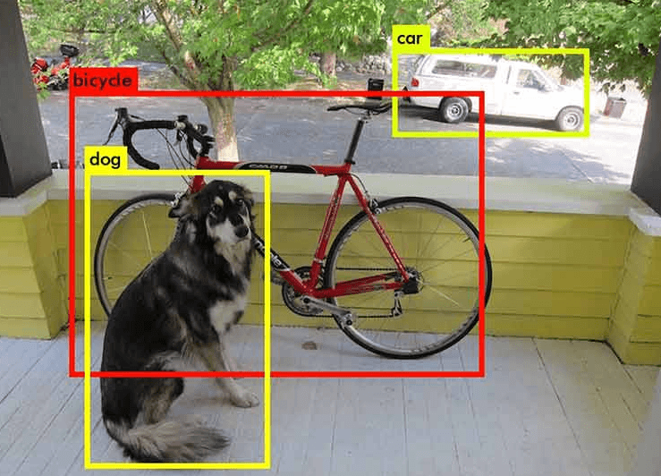
This is one of the most fundamental tasks in computer vision, one step up in complexity to image classification and one step down to image segmentation. Recent advances in deep learning have yielded extraordinarily accurate object detection models with countless practical applications.
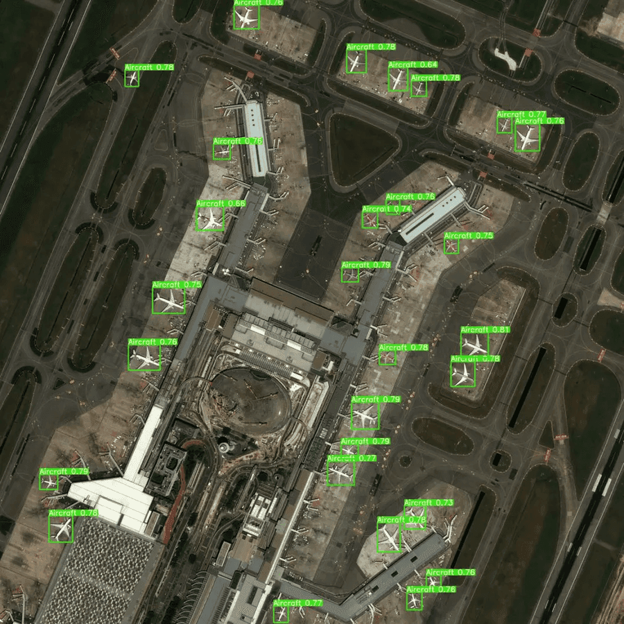
In this post I will summarize and discuss the most important architectures for tackling object detection with deep learning.
Overview of Architectures
Object detection architectures can be broadly grouped into two main categories: two-stage detectors and one-stage detectors.
Two-stage detectors
Two-stage detectors first generate region proposals where objects might be located, then refine these proposals and classify the objects within them. These methods prioritize accuracy over speed.
| Architecture | Strengths | Weaknesses | Use Cases |
|---|---|---|---|
| R-CNN | High accuracy, foundational approach | Very slow, computationally expensive | Research, detailed image analysis |
| Fast R-CNN | Faster than R-CNN, shared computation | Still slower than modern methods | Applications where accuracy is key |
| Faster R-CNN | High accuracy, end-to-end training | Slower than one-stage detectors | Tasks requiring precise localization |
| Mask R-CNN | Adds instance segmentation, very accurate | Computationally intensive | Object detection + segmentation |
One-stage detectors
One-stage detectors perform object detection in a single pass, directly predicting class probabilities and bounding boxes from the input image. These methods are faster but may sacrifice some accuracy compared to two-stage detectors.
| Architecture | Strengths | Weaknesses | Use Cases |
|---|---|---|---|
| YOLO | Real-time detection, fast and efficient | Less accurate for small objects | Real-time applications, robotics |
| SSD | Good speed-accuracy trade-off, multi-scale | Less precise than two-stage detectors | Mobile applications, embedded systems |
| RetinaNet | Focal Loss improves detection of hard cases | Slower than YOLO, complex training | Detection in challenging scenarios |
| In this post I will dive deep into YOLO architectures. |
YOLO
YOLO, which stands for "You Only Look Once," is a widely recognized real-time object detection algorithm that has become a cornerstone in the field of computer vision. First introduced in 2016, YOLO was revolutionary for its speed, outperforming all other object detectors available at the time.
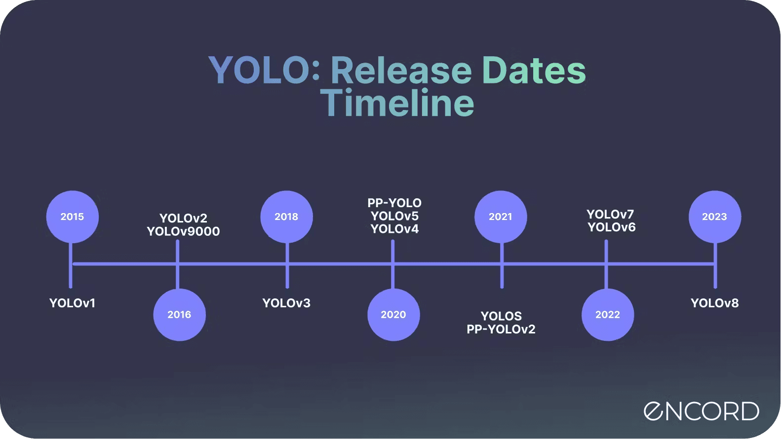
Since the original release, YOLO has undergone several iterations, each bringing significant advancements in performance and efficiency. Let's see an overview of the different versions:
| YOLO Version | Main Innovations | Authors / Research Group | Release Date |
|---|---|---|---|
| YOLO | First real-time object detection algorithm; single-stage detection. | Joseph Redmon et al. | 2016 |
| YOLOv2 | Improved accuracy, multi-scale detection, anchor boxes. | Joseph Redmon et al. | 2016 |
| YOLOv3 | Multi-scale predictions, better performance on small objects, Darknet-53 backbone. | Joseph Redmon and Ali Farhadi | 2018 |
| YOLOv4 | CSPDarknet backbone, mosaic data augmentation, self-adversarial training. | Alexey Bochkovskiy, Chien-Yao Wang, et al. | April 2020 |
| YOLOv5 | Improved usability, PyTorch implementation, auto-learning bounding boxes. | Ultralytics | June 2020 |
| YOLOv6 | Faster inference, more compact model architecture, optimized for edge devices. | Meituan | 2022 |
| YOLOv7 | Efficient Layer Aggregation Networks, advanced model scaling, cross mini-batch norm. | Chien-Yao Wang, Alexey Bochkovskiy, et al. | July 2022 |
| YOLOv8 | Enhanced usability, ease of training and deployment, more accurate and faster. | Ultralytics | January 2023 |
| YOLOv9 | Further speed and accuracy improvements, enhanced feature extraction techniques. | Ultralytics (anticipated future version) | February 2024 |
YOLO Step by Step
- YOLO divides the input image into an
S×Sgrid (for example,7x7). Each grid cell is responsible for detecting objects whose center falls inside the cell.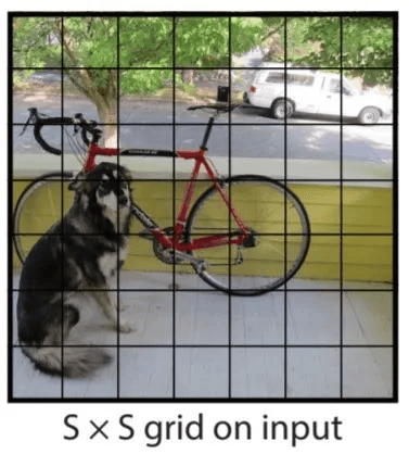
- For each grid cell, YOLO predicts several bounding boxes (usually 2 to 5), along with a confidence score for each box. This confidence score reflects:
- How confident the model is that a box contains an object.
- How accurate the predicted bounding box is relative to the actual object’s position.

Each bounding box consists of five predictions:
- x: x-coordinate of the center of the box (relative to the grid cell).
- y: y-coordinate of the center of the box.
- w: width of the box (relative to the whole image).
- h: height of the box.
- Confidence score (how certain the model is about the presence of an object (any object) in that box).
- per-class score: probability of each class
- The final score for a bounding box is the product of the object confidence score times the class probabiliyt
- Non-maximum suppression is employed eliminate overlapping boxes. This step helps retain the best bounding box for each detected object, based on the confidence score, while discarding redundant boxes.
A high level summary is: YOLO makes a single pass over the image, proposing a set of bounding boxes for each grid that is subsequently cleaned by non-max suppression.
A few remarks:
- Advanced versions of YOLO actually set predefined shapes for the boxes predicted for each grid (anchor boxes). These predefined shapes could be more elongated, or tall, etc ; so that each specific anchor box specialises on detecting boxes of a specific shape. The model predicts modifications to these predefined shapes, rather than predicting the bbox shapes from scratch.
- If there are many small objects within the same grid, YOLO may struggle or even be incapable of detecting them. The max number of objects per cell grid is bounded by the number of boxes predicted per cell.
Aligning the data
There's a significant gap between the simple bounding box annotations we typically have in object detection datasets (e.g., COCO, Pascal VOC) and the high-dimensional output predicted by a model like YOLO. Here’s the step-by-step process of how we adapt the simple dataset annotations (bounding boxes) to YOLO’s output format:
- Convert bbox format: First, we convert the bounding box coordinates from the typical
(xmin, ymin, xmax, ymax)format to the center format(x_center, y_center, w, h), more suitable for YOLO architecture that predicts the center of the box as offsets from grid cell centers. - Assign objects to grid cells: For each object (bounding box), we assign it to a grid cell based on the location of the center of the bounding box. If the center of the object’s bounding box falls within a particular grid cell, that grid cell becomes responsible for predicting that object.
- Match bboxes to anchor boxes: Next, we match the ground truth bounding boxes to the predefined anchor boxes (or learned anchors) used by YOLO. We pick the anchor box that maximizes the IoU with the ground truth box, and assign it as responsible of predicting that object. This step is crucial because YOLO predicts adjustments to anchor boxes, rather than the actual bounding boxes.
- Encode bounding box adjustment: Once we have matched the ground truth bounding box to an anchor box, we need to encode the offsets the model should predict.
- Encode class labels: For each grid cell and its assigned bounding box, we encode the object’s class label as a one-hot vector where the actual class is set to 1.
- Confidence score: For the bounding box assigned to an object, we set the confidence score to 1 (indicating an object is present). For all other anchor boxes in the grid cell that aren’t assigned to an object, the confidence score is set to 0.
The loss function
YOLO uses a multi-part loss function that includes terms for:
- Bounding box regression (localization loss): primarily based on MSE over the bounding box coordinates (a loss suitable for a regression task)
- Confidence score (objectness loss): Also based on MSE
- Class prediction loss (classification loss): Usually a variant of cross-entropy loss on the predicted classes.
The actual loss looks a little more daunting, but the base ideas I just shared stand:
 Notes:
- Non-max suppresion doesn't take part of the loss calculation, it's a post-processing step
- Advanced version of YOLO keep being released every year
Misc
Benchmarks
The most popular benchmark is the Microsoft COCO dataset.
 The most popular benchmark datasets for object detection include:
- COCO (Common Objects in Context): A widely used dataset that contains over 330,000 images with 80 object categories. It includes annotations for object detection, segmentation, and keypoint detection.
- PASCAL VOC (Visual Object Classes): This dataset has been influential in object detection research, containing images from 20 object categories. The challenges associated with this dataset have been used to evaluate various detection algorithms since 2007.
- ImageNet: Primarily known for image classification, ImageNet also provides a large number of annotated images for object detection tasks, particularly through its ImageNet Detection Challenge.
Metrics
Different models are typically evaluated according to a Mean Average Precision (MAP) metric. It combines the concepts of precision and recall across different object classes and detection thresholds.
- Precision: The proportion of true positive detections (correctly detected objects) among all positive detections (both true and false positives). If you have many classes, you can calculate precision for each class grouping all other classes as the negative class.
- Recall: The proportion of true positive detections among all actual objects (true positives plus false negatives). Can also be calculated per class.
- Average Precision is the area under the Precision-Recall curve for a specific class. You get one per class. The precision recall curve is made of the precision,recall pairs at different confidence thresholds e.g. confidence > 0.5 ; etc.
- mAP is the mean of the Average Precision (AP) values computed for each class in the dataset. It provides a single metric that summarizes the model's performance across all classes.
mAP_{50-95}: mAP is computed for each class and for each IoU threshold in a range from are computer at 10 IoU tresholds (0.50 to 0.95) for each class.
Example:
- Imagine you have 3 classes: Person, Car, and Dog.
- Ground Truth: 3 persons, 2 cars, 1 dog in an image. Predictions:
- 2 boxes for Person: 1 is correct (IoU ≥ threshold), 1 is incorrect (IoU < threshold).
- 1 box for Car: Correct (IoU ≥ threshold).
- 2 boxes for Dog: 1 is correct, 1 is misclassified (e.g., as Person).
Tangent tasks and variations
Traditional object detection typically involves predicting bounding boxes in 2D RGB images, but there are several variants and extensions of this task that address different scenarios and data types. Here are some notable ones:
- Non-Square Bounding Boxes: Traditional object detection often uses square or rectangular bounding boxes, but variants exist that can predict non-square (e.g., rotated) bounding boxes. This is useful for objects that are not aligned with the image axes, like vehicles or certain shapes.
- 3D Object Detection: This variant involves detecting objects in 3D space, often using depth information from sensors like LiDAR or stereo cameras. 3D bounding boxes are used to represent the position, orientation, and size of objects in 3D coordinates.
- Keypoint Detection: Instead of just predicting bounding boxes, this approach identifies specific points of interest on an object (like facial landmarks or body joints). It is particularly useful in applications like pose estimation and facial recognition.
- Video Object Detection:This variant extends detection to video sequences, requiring models to track and detect objects over time. Techniques often involve motion estimation and temporal consistency.
- Multi-Label Object Detection: In this variant, an object can belong to multiple classes, allowing for more complex scenarios like detecting an object as both "person" and "athlete" in a sports context.
- Point Cloud Object Detection: For data obtained from 3D sensors (like LiDAR), models are designed to directly process point clouds, detecting objects based on the 3D coordinates of points.
- Few-Shot and Zero-Shot Object Detection: These approaches aim to detect objects with very few or no training examples. Few-shot detection learns from a small number of labeled samples, while zero-shot detection attempts to identify unseen classes using semantic information.
Practical Example: Checkbox Detection
For a hands-on comparison of traditional computer vision vs. YOLO for a real object detection task, check out my post on Checkbox Detection: OpenCV vs YOLO. It demonstrates how YOLO can be trained with just 5 images to detect and classify checkboxes in scanned documents.