Review and Summary of Deep Learning Specialization from DeepLearning

Introduction
At work, we enrolled into the Deep Learning Specialization from DeepLearn.ai via Coursera. Even though this is quite a basic level course, I decided to give it a try and take the chance to revise my foundations.
There is quite a lot of praise online for this course. It lacked depth, there were no structured course notes (just videos), and the above all author kept embarking on lengthy "intuitive" explanations aimed at people who did not take a proper calculus course. That said, I think it's great as a very comprehensive overview of the field.
If you graduated from university, or if you already have knowledge on neural networks, this course is probably too basic for you. Nevertheless, even though I did not learn almost that many new things, it was a great chance to revisit basic concepts and get a certificate that can be showcased in LinkedIn. Moreover, fifth part (sequence data) was quite new to me, never having delved deeper into certain topics.
Below is a summary of the contents developed in the specialisation, based on my notes and takeaways.
Course 1: Neural Networks and Deep Learning
Week 1: Introduction to Deep Learning
This is a very relaxed welcome unit. Neural networks are loosely presented as systems that can learn to solve tasks involving many inputs and outputs, and excel at dealing with unstructured data (images, audio, text)
Structured data, on the other hand, is highly organized and easily searchable. It is typically stored in relational databases or spreadsheets, where the data is arranged in rows and columns with specific data types.
The teacher emphasizes that neural networks performance scale with the amount of data, and in general are very data-hungry. They are able to surprass traditional ML methods (such as SVM), but they do require substantial quantity of data samples.
Week 2: Basics of Neural Network programming
Logistic Regression
Binary classification is exemplified with the task of predicting, giving an input image, whether it is a cat picture or a doc picture.
In this example, RGB images of 64x64 pixels are rearranged into a flat vector of 12288 elements. This is the dimension of the inputs in this setup for this task.
Given a dataset of m cat-dog pictures and their labels, they are arranged into matrixes as follows:
X: A n x m matrix where each column is one of the training inputs, and n is the leng th of the inputs (12288 for this example)
Y: A 1 x m matrix where each column is the label of one of the training inputs.
The teaches introduced a well known, simple classification method: Linear Regression.
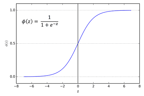
Given an input x (e.g. a dog-cat image), it is meant to predict \hat(y) where 0 <= \hat(y) <= 1 by applying a linear function followed by a sigmoid function to squeeze the output of the linear function to [0,1]
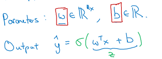 The parameters of the model are
 w and b. Recall the shape of the sigmoid function here:
 In order to use the training set of
 m labeled samples to tune the parameters w and b , a few concepts are introduced:
- The loss (error) function L, which tells how different a model prediction is from its labelled ground truth. Since this is a binary classification problem, the Binary Cross-Entropy Loss is introduced
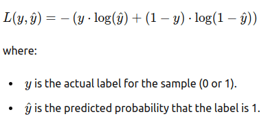
- The cost function J is the sum of the loss over the entire training set for any given choice of parameters

- Gradient descent is an iterative method used to find w and b that minimize J(w,b). It consists of updating w and b on each iteration by substracting the derivative of J with respect to the parameters. By moving the paremeters in the direction opposite to the gradient, the cost function value is driven down and the model should become better at predicting the training labels. A hyperparameter alpha, the learning rate, governs the strength of the parameter update on each iteration.
Here, the teacher goes into A LOT of extra-boring examples trying to impress the meaning of a derivative without actually diving into the math. Having taking in-depth courses of calculus at university, this was a stump.
It's actually quite simple. f'(a) gives an approximation of how f changes if you slightly modify a. Say f'(a)=2, then f'(a+delta) ~= f(a) + 2*delta
It becomes a little more interesting when we talk about derivatives in a computational graph. Here a system takes three inputs, a, b and c ; makes a few intermediate computations u and v and finally produces an output J

The key point here is that, if we want to know the derivative of J with respect to the inputs (e.g. b or c), we need to apply the chain rule and go through the intermediate nodes.
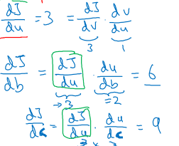
In the context of logistic regression, we can calculate the derivative of the loss L by writing it as a computational graph:

This example has inputs with size 2 (thus two weights). We need the derivative of L wrt to the parameters w_1, w_2 and b.
In order to do so, we first need the intermediate derivatives:
da = D L(a,y) / D a = -y/a + (1-y)/(1-a)
dz = DL/Dz = DL/Da * Da/Dz = da * a*(1-a) = a-y
dw1 = DL/dw1 = DL/z * Dz/Dw1 = dz * x1
After calculating the final derivative, we can update
w1 := w1 - alpha * dw1
And do the same for the other parameters.
To scale this up to m examples, we need to calculate the derivatives of the cost function J. Since the derivative of a sum is the sum of the derivatives, this is quite straightforward.

This section concludes with a snippet of code that makes an iteration of gradient descent, calculating the cumulative gradient over the entire training set. Notice that this would have to be repeated iteratively until convergence.
Also notice that n=2 meaning that x is just x1 and x2. If n is large, this code is inefficient. Vectorization would have to be used to get rid of for loops.
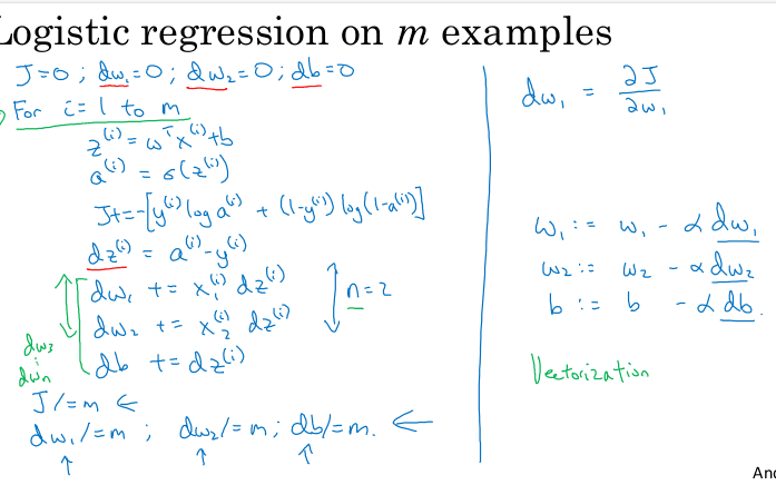
Vectorization
Replacing explicit for loops by matrix/vector built in operations can considerable speed up your algorithms both in GPU and CPU.
Examples:
- In order to multiply a matrix by a vector, use
np.dot(A,v) - In order to apply the same function to each element in a vector
v, use built-in operations that are very efficientnp.exp(v),np.log(v),np.abs(v),np.maximum(v,0),v**2,1/v - use
np.sum,
This is mostly exemplified by the assignment 1 tasks, which you can check out in my GitHub.
Week 3: Shallow Neural Networks
Neural networks
There's a very verbose intro here just to explain the concept of a fully connected neural network and notation.
Basically it is a sequence of layers, each all consecutive layers are fully connected by parameters w.
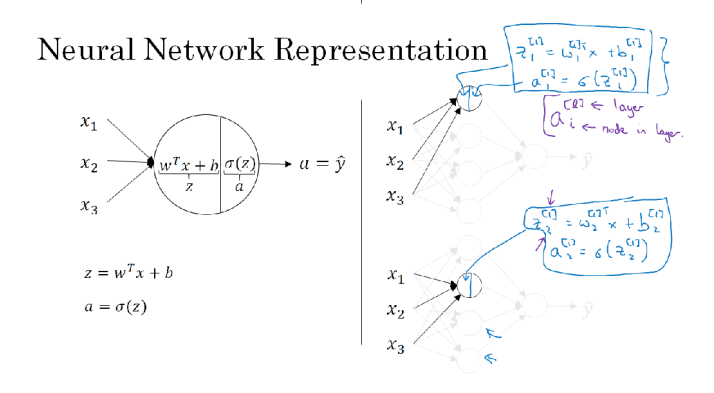 A neuron computes a weighted sum using a parameter
 w of all its parameters, adds a bias parameter b and then applies a non-linear activation function such as sigmoid
We are introduced to different choices of activation functions. The rule of thumb is: use ReLu, unless you're on the last output layer of a binary classification task, there you can use Sigmoid.
Non-linearities are crucial to represent complex functions, otherwise the entire network collapses into a single linear function!
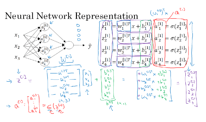
Here's a FCN with two layers (the input layer doesn't count). The notation is defined as follows:
**z^\[i\]\_j**: The output of the jth neuron at the ith layer.**a^\[i\]\_j**: Activation function applied to the previous value**w^\[i\]\_j**: weight to connect neurons in layer{i-1}to neuronjin layeri**b^\[i\]\_j**: bias used by neuron j at layer i These values are stacked together to form matrixes that allow for efficient vectorization:**a^\[i\]**,**z^\[i\]**all activations from layer i**W^\[i\]**: Weights that connect layer{i-1}to layer{i}**b^\[i\]**: all biases of neurons at layer i
Thus we can rewrite the equations in vectorized form, where the (i) superscript means sample number i. We can stack all samples together to vectorize this as well.
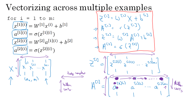
Gradient Descent for Neural Netoworks
The author presents pseudocode for a single-hidden-layer neural network, and we can see it's quite similar to logistic regression:
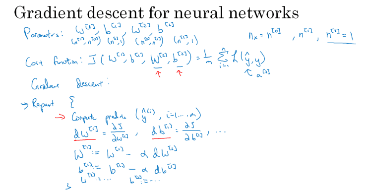 The derivatives of the activation functions are:
- Sigmoid:
	g(z)  = 1 / (1 + np.exp(-z))
	g'(z) = (1 / (1 + np.exp(-z))) * (1 - (1 / (1 + np.exp(-z))))
	g'(z) = g(z) * (1 - g(z))
- RELU
    g(z)  = np.maximum(0,z)
    g'(z) = { 0  if z < 0
              1  if z >= 0  }
The forward propagation goes as follows:
Z^1 = W1A0 + b1    # A^0 is X
A^1 = g1(Z1)
Z^2 = W2A1 + b2
A^2 = Sigmoid(Z2)   # Sigmoid because the output is between 0 and 1
Finally, let's do backpropagation:
dA^2 = -Y/A^2 + (1-Y)/(1-A^2)   # Calculus
dZ^2 = DL/DZ^2 = DL/DA^2 * DA^2/DZ^2 = dA^2 * (A^2 * (1-A^2)) = A^2 - Y^2
dW^2 =  dZ^2 * DZ^2/DW^2 = (dZ^2 * A^1.T)/m
db2 = Sum(dZ2) / m
dZ1 = (W2.T * dZ2) * g'1(Z1)  # element wise product (*)
dW1 = (dZ1 * A0.T) / m   # A0 = X
db1 = Sum(dZ1) / m
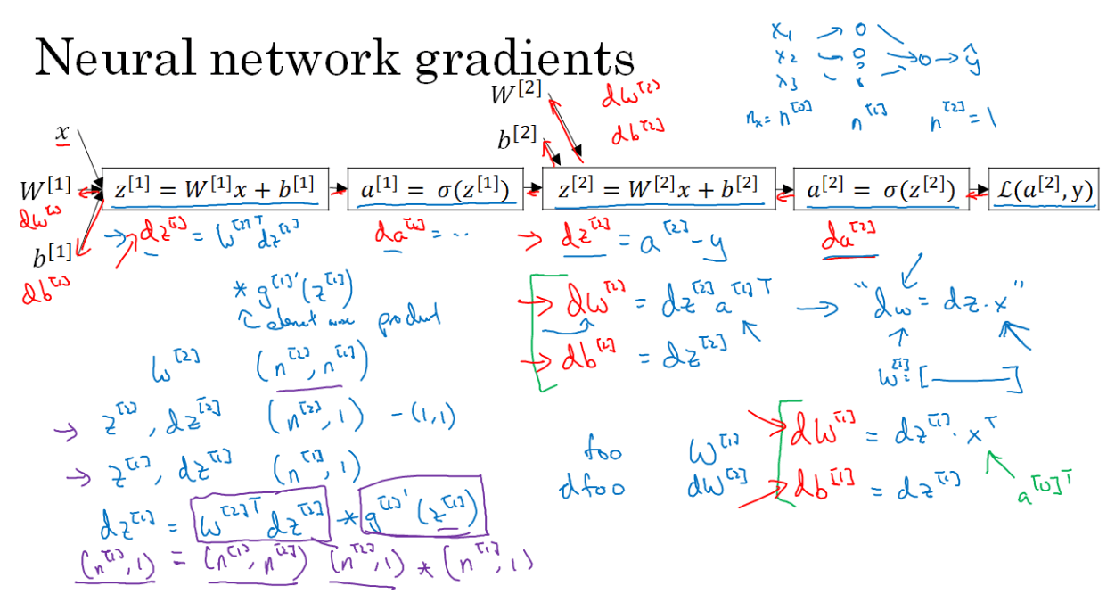
Mira el video de la intuition por que:
- no entiendo por que involucra ms si la loss no es la J
- no entiendo por que transpuestas, asumo que algo de calculo de matrices
- no entiendo por que Sum en las derivadas de las bs
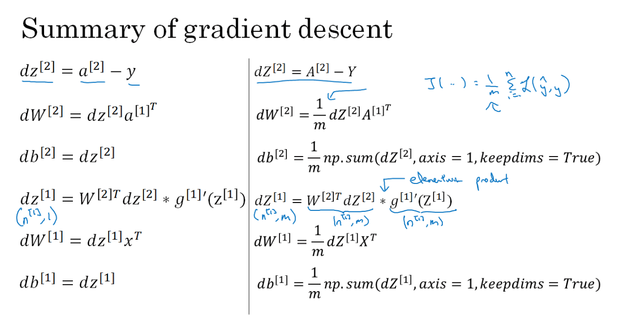 Left: single sample - Right: All training set at once
So basically you are calculating the direction you have to go to reduce the error for each training sample, and the you average out that direction to update the weights.
Random Initialization of Parameters
What happens if we initialize our NN to have all zero weights?
It's possible to construct a proof by induction that if you initialize all the values of w to 0, each neuron in a given layer will compute the same output because they all start with the same weights and biases. Consequently, the gradients for these neurons will also be identical during backpropagation. This symmetry means that each neuron in a layer will continue to update in the same way, preventing the network from breaking symmetry and learning diverse features. Essentially, the neurons in each layer will remain identical throughout the training process, significantly limiting the model's capacity to learn.
The solution to this is to initialize the parameters randomly to small numbers, e.g.:
W^1 = np.random.randn((2,2)) * 0.01
Large numbers would cause activations such as sigmoid or tanh to saturate, making learning slow.
link to the assignment 3.
Week 4: Deep Neural Networks
A deep NN is a NN with three or more layers:
L: Number of layersn^[l]: number of neurons at layerl(n[0]number of inputs,n[L]number of outputs)g^[l]: activation function at layerlz^[l] = W^[l] * a^[l-1] + b^[l]has shape(n[l],1)a^[l] = g^[l](z^[l]): activation at the layerlhas shape `(n[l],1)W^[l]: weights that connect layerl-1to layerlhas shape(n[l],n[l-1])b^[l]: biases of layerl, shape is(n[l],1)x = a[0],a[l] = y'
Vectorized for the entire training set:
m: number of training samplesZ^[i] = W^[i] X + b^[i]has shape(n[i],m)Xhas shape(n[0],m)(i.e. each sample is a column, contrary to the conventions that the rest of the world uses)A[0]=XA[l]=g^[l](Z^[l])has shape(n[i],m)dZ^[l]anddA^[l]will have shape(n[i],m)
Why use deeper networks? earlier layers of the neural network can detecting simple functions, like edges and then composing them together in the later layers of a neural network so that it can learn more and more complex functions.
This is the typical intuition for hierarchical feature extraction in CNNs (I don't actually think it applies to dense layers though)
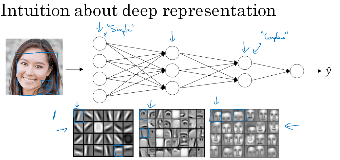
Another example with speech recognition. The first level of a NN may detect low lavel audio wave forms and basic phonemes. Later layers may compose this together.
This in some way emulates what our brain does.
Generic forward and backward functions (vectorized to all samples)
-
Pseudo code for forward propagation for layer l:
Input A[l-1] Z[l] = W[l]A[l-1] + b[l] A[l] = g[l](Z[l]) Output A[l], cache(Z[l]) -
Pseudo code for back propagation for layer l:
Input da[l], Caches dZ[l] = dA[l] * g'[l](Z[l]) dW[l] = (dZ[l]A[l-1].T) / m db[l] = sum(dZ[l])/m # Dont forget axis=1, keepdims=True dA[l-1] = w[l].T * dZ[l] # The multiplication here are a dot product. Output dA[l-1], dW[l], db[l] -
Cross entropy loss function is:
dA[L] = (-(y/a) + ((1-y)/(1-a)))
Parameters and Hyperparameters
- The parameters of the network are
wandband they are optimized via backpropagation - Hyperparameters are higher level parameters of the algorithm such as:
- The learning rate (alpha)
- The number of iterations until convergence
- The number of hidden layers
Land the number of hidden units per hidden layer - The choice of activation functions
Hyperparameters are often optimized by trying a few combinations of them and checking which one works better (this is actually developed in depth in the next course)
I cannot recommend this video and its sequel more: https://www.youtube.com/watch?v=Ilg3gGewQ5U.
Course 2 - Improving Deep Neural Networks: Hyperparameter tuning, Regularization and Optimization
Week 1: Practical Aspects of Deep Learning
Train / Validation / Test set
In machine learning, we usually iterate through the loop:
Idea -> Code -> Experiment -> Repeat
During the process of defining the hyperparameters of a model, it is recommended that the available data is split into three sets:
| Data partition | Purpose | Size |
|---|---|---|
| Training set | Optimizing model parameters | 60 to 98 % |
| Validation set AKA dev set | Optimizing model hyperparameters | 20 to 1% |
| Test set | Provide an unbiased estimation of performance | 20 to 1% |
| If size of the dataset is greater than 1M we may use 98/1/1 or even 99.5/0.25/0.25 |
- Train and validation set must come from the same distribution
- The dev set is used to try out trained models with different hyperparameters, in order to define what is the best hyperparameter configuration
- It is ok to only have validation set without testing set if you don't need an unbiased estimation of performance. People call the validation set "test set" in this setup (although it is misleading).
Bias and Variance
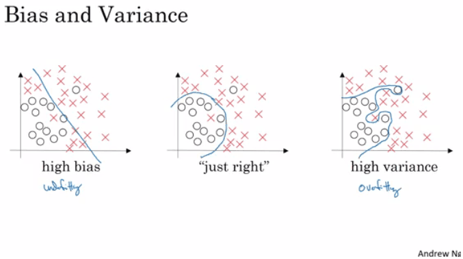
- A model that underfits has high bias
- e.g. training error doesn't go down near the optimal classifier error
- A model that overfits has high variance
- big gap between training and validation error.
- A good model strikes a good balance between bias an variance
- training and validation error closer to the optimal classifier
A basic recipe for Machine Learning is:
- If your algorithm has high bias
- Make your NN larger (more hidden units or layers) - This never hurts. Still I advise starting smaller.
- Try out different models
- Train for longer
- Use a different optimization algorithm
- If your algorithm has high variance
- Add more data
- Regularization
- A different model
Historical note: In traditional ML we usually talk about the bias/variance tradeoff, but in the deep learning world we can usually try to improve either without making the other worse.
Regularization
Regularization techniques reduce overfitting and therefore reduce variance.
Weight Decay
We can apply regularization to the parameters of the model by penalising large weights in the cost function. In order words, we try to keep the model from becoming "too complex". This is sometimes called weight decay.
The cost function looks like this when we add regularization, where lambda is the regularization hyperparameter:
J(w,b) = (1/m) * Sum(L(y(i),y'(i))) + (lambda/2m) * Sum((||W[l]||)
We can use either L1 (Aka Lasso) or L2 (aka Ridge) norm:
-
L1 encourages sparsity in
w, potentially making for a smaller and more efficient model. It is preferred when you think some features are irrelevant.||W|| = Sum(|w[i,j]|) -
L2 is much more popular. It encourages smaller but non-zero weights.
`||W||^2 = Sum(|w[i,j]|^2)
Notice that the gradient of L2 is proportional to 2 * lambda* w_i , meaning that larger weighs experience a proportionally large force pulling them towards zero. This proportionality results in a more uniform shrinkage across all weights. Large weights are reduced significantly, but small weights are reduced less. This uniform shrinkage does not typically result in exact zeros but rather smaller weights overall.
On the other hand, the gradient of L1 is a constant value (lambda or -lambda), except at zero where it's undefined. This constant force encourages weights to move towards zero by a fixed amount, regardless of their size. As a result, small weights can be reduced to exactly zero, creating sparsity.
So, if we have a new J with L2 norm, the new backpropagation update is:
dw[l] = (old backprop value) + lambda/m * w[l]
Thus the new update step is:
w[l] = w[l] - learning_rate * dw[l]
     = w[l] - learning_rate * ((old backprop value) + lambda/m * w[l])
     = w[l] - learning_rate * (from back propagation) - (learning_rate*lambda/m) * w[l]
The new term shrinks w[l] proportionally to w[l] itself and to the lambda parameter, pulling it towards zero. This is, this penalizes large weights and effectively limits the freedom in your model.
How does weight decay helps?
- Large weights can make the model respond with high sensitivity to the input features. This sensitivity allows the model to fit the training data very closely, including noise. In other words, it makes it easy to memorize instead of learn. It also results in more complex decision boundaries.
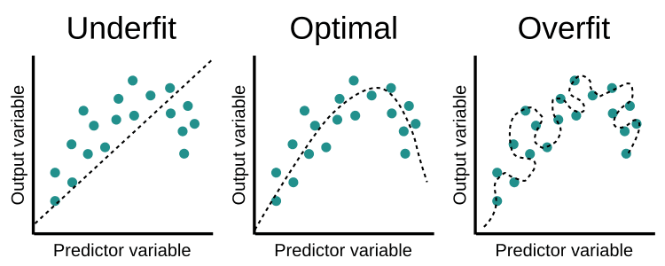
- Smaller weights constrain the model, reducing its sensitivity to individual input features. This results in a smoother, more general decision boundary that captures the underlying patterns of the data rather than the noise.
Imagine fitting a polynomial to data points:
Dropout
The dropout regularization eliminates some neurons (along with all their incoming and outgoing edges) on each iteration based on a probability.
The usual implementation is called Inverted Dropout:
keep_prob = 0.8   # 0 <= keep_prob <= 1
l = 3  # this code is only for layer 3
# the generated number that are less than 0.8 will be dropped. 80% stay, 20% dropped
d3 = np.random.rand(a[l].shape[0], a[l].shape[1]) < keep_prob

a3 = np.multiply(a3,d3)   # keep only the values in d3

# increase a3 to not reduce the expected value of output
# (ensures that the expected value of a3 remains the same) - to solve the scaling problem
a3 = a3 / keep_prob
To ensure that the scale of the output remains the same, the outputs of the remaining neurons are scaled up. This scaling factor compensates for the dropped neurons, keeping the expected value of the outputs constant.
During inference, dropout is not applied, and the entire network is used. No scaling is needed because the dropout is not active.
Dropout can have different keep_prob per layer.
Why does it work?
- Can't rely on any one feature, so have to spread out weights. Otherwise neurons can become overly reliant on specific other neurons, leading to a fragile model.
- By randomly dropping out neurons during training, dropout forces the network to learn more robust and independent features.
- Since neurons cannot rely on specific other neurons, they must learn redundant representations of features. This redundancy makes the model more robust to changes in the input data.
- It works very well on CV tasks, empirically.
Data augmentation
Often used in CV data, it involves flipping, rotating, distorting the images. This makes the model able to generalize better to slight changes.
Early stopping
In this technique we plot the training set and the dev set cost together for each iteration. At some iteration the dev set cost will stop decreasing and will start increasing. We pick the point where the validation set is lowest.
Model Ensembles
- Train multiple independent models.
- At test time average their results.
While ensembling is commonly associated with traditional machine learning methods like decision trees and support vector machines, it is also a powerful technique in deep learning.
Normalizing the inputs
If you normalize your inputs this will speed up the training process a lot. Substract the mean of the training set from each input and divide by the variance of the train set.
These steps should be applied to training, dev, and testing sets (but using mean and variance of the train set).
If we don't normalize the inputs our cost function will be deep and its shape will be inconsistent (elongated) then optimizing it will take a long time.
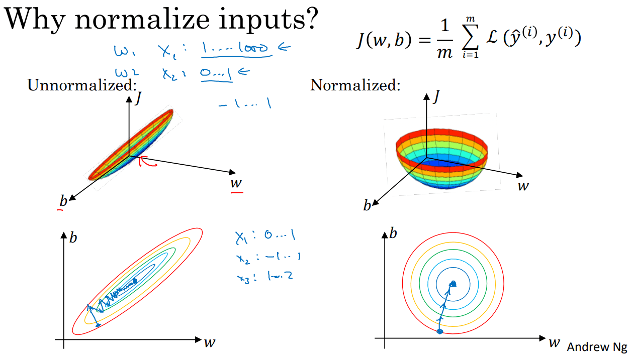
Normalized inputs allow for a larger learning rate and optimization will thus be faster.
Vanishing / Exploding gradients
The Vanishing / Exploding gradients occurs when your derivatives become very small or very big, especially in very deep networks. It will take a long time for gradient descent to learn anything, if able to learn at all.
Definition:
- In neural networks, the learning process involves adjusting the weights using gradient descent, which relies on the gradients (partial derivatives) of the loss function with respect to the weights.
- When gradients are very small, the updates to the weights become minuscule. This means that the weights change very slowly, and the network learns at a very slow pace, potentially getting stuck and not learning effectively.
- When gradients are very large, the updates to the weights become very large as well. This can cause the weights to grow uncontrollably, leading to numerical instability and making the network unable to converge.
Causes:
- Functions like the sigmoid or tanh compress a wide range of input values into a small range (0 to 1 for sigmoid, -1 to 1 for tanh). When many layers use these functions, the gradients get multiplied several times, causing them to shrink exponentially and approach zero.
- Improper initialization can exacerbate the vanishing gradient problem. If initial weights are too small, the gradients can vanish even faster. If weights are too big, gradients can explode.
- Deep networks. The more layers there are, the more times the gradients are multiplied, increasing the likelihood of them becoming extremely small.
Solutions:
(1) Smart initialization of weights. Xavier (Glorot) set the initial gradients so that they are in a reasonable range.
Xavier initialization achieves this balance by setting the initial weights according to the size of the previous layer. Specifically, it uses a distribution with a variance that is inversely proportional to the number of input neurons in the layer.
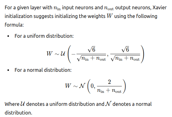
Pytorch uses a similar approach by default for linear and convolutional layers.

Others:
- Batch normalization
- Gradient clipping
- Residual networks
- Auxiliary heads
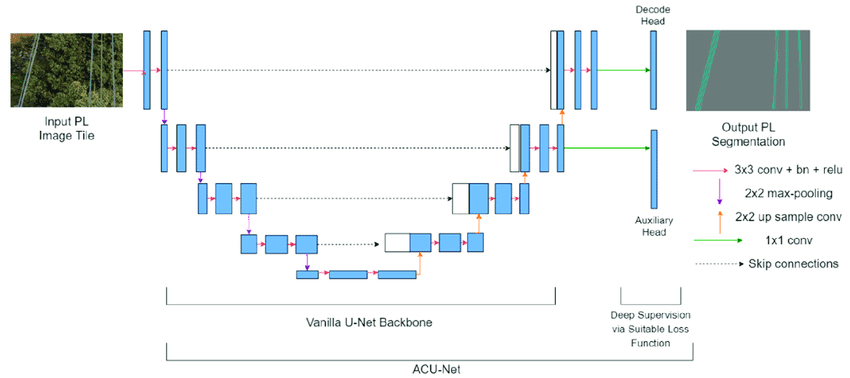 Skip connections
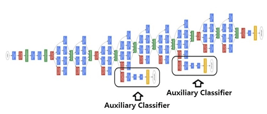 Auxiliary heads
Gradient checking
This seems only relevant if you're implementing your own architecture and optimization code. Not the most common situation of a ML practitioner.
It involves approximating the derivatives of the weights of a specific sample, and checking that your algorithm is calculating them correctly.
Week 2 - Optimization algorithms
Mini-batch gradient descent
Instead of calculating the gradient over the entire dataset (which could be HUGE and potentially intractable), we can calculate the gradient over a small sample of the training dataset to approximate the gradient, and make more frequent updates to the weights.
- Batch gradient descent: Calculate the gradient over the entire dataset (what we have done so far)
- Mini-batch gradient descent: Run gradient descent on mini batches. Works much faster in large datasets.
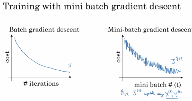 MBGD has ups and downs, but the updates are much more frequent.
Definitions:
- Iteration: Each process of calculating the gradients and updating the weights. In MBGD, it means going through a mini batch and updating the weiths.
- Epoch: Going over each sample in the entire training dataset. In MBGD it'd involve many iterations.
The mini batches could be either:
- Randomly sampled with replacement on each iteration. These samples can overlap with elements from previous iterations because sampling is done with replacement (Stochastic Mini-Batch Gradient Descent). SGD often refers to having batch size just 1.
- Calculated by slitting the dataset into non-overlapping mini-batches (Deterministic Mini-Batch Gradient Descent)
| Method | batch size | Pros | cons |
|---|---|---|---|
| batch gradient descent | m | accurate steps | takes too link per iteration, maybe intractabe |
| mini batch gradient descent | >=1 ; <= m | faster learning bc you have vectorization and more regular weight updates | may not converge, requires tuning LR properly - need to tune mini batch size hyperparameter |
| Stochastic gradient descent | usually 1 | very noisy gradient requiring small learning rate ; may diverge ; loses vectorization advantage | |
| mini bach size: |
m<2000=> use batch gradient descentm<2000=> use a power of 2 as batch size e.g. 64, depending on your GPU memory
Exponentially weighted averages
This is a mathematical concept, forget about NN now.
Exponential weighted averages (EWAs), also known as exponential moving averages (EMAs), are used to smooth out data series to highlight trends by giving more weight to recent observations while exponentially decreasing the weights of older observations.
The idea behind exponential weighted averages is to apply weights that decay exponentially. More recent data points have higher weights, and the weights decrease exponentially as the data points get older.
The exponential average v(t) at time t of series theta is given by:
v(t) = beta * v_{t-1} + (1-beta) * theta_t
beta is the smoothing factor, and (1-beta) controls the rate at which the influence of past observations decays.
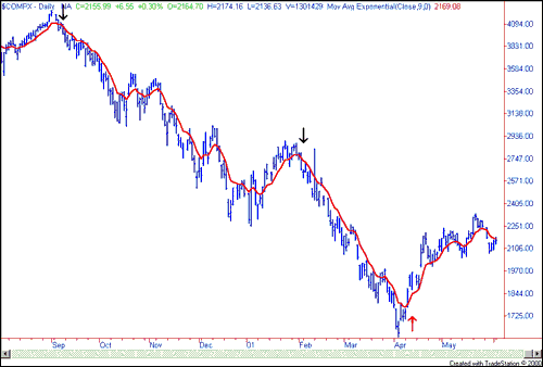 Example of a time series and its EWAs
The average starts at v(0)=0 which gives a bias and shifts the average at the beginning, making it inaccurate. We can correct this bias by using the following equation:
v(t) = (beta * v(t-1) + (1-beta) * theta(t)) / (1 - beta^t)
As t becomes larger the (1 - beta^t) becomes 1
Momentum
Let's now use this mathematical tool in mini batch gradient descent. We can smooth out the gradients obtained by mini-batch gradient descent using a EWA, reducing oscillations in gradient descent and making it faster by following a smoother path towards minima.
Best beta hyperparameter average for our use case is between 0.9 and 0.98 which will average between 10 and 50 last entries.
The update rule then becomes:
vdW = 0, vdb = 0
on iteration t:

	compute dw, db on current mini-batch

	vdW = beta * vdW + (1 - beta) * dW
	vdb = beta * vdb + (1 - beta) * db

	W = W - learning_rate * vdW
	b = b - learning_rate * vdb
So instead of updating via the last weight, we use the EWA, which is smoother and pushes towards keeping the tendency of previous updates.
RMSprop
Root Mean Square Prop, is another technique to speed up gradient descent. It keeps a rolling average of the square gradients:
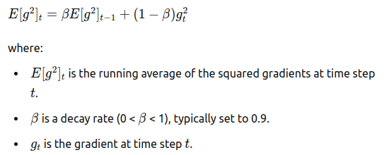
This square average is used to normalize the learning rate on each weight update:
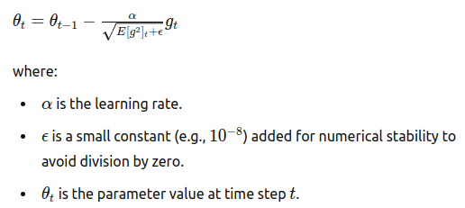 In pseudocode:
sdW = 0, sdb = 0
on iteration t:
	# can be mini-batch or batch gradient descent
	compute dw, db on current mini-batch

	sdW = (beta * sdW) + (1 - beta) * dW^2  # squaring is element-wise
	sdb = (beta * sdb) + (1 - beta) * db^2  # squaring is element-wise
	W = W - learning_rate * dW / sqrt(sdW)
	b = B - learning_rate * db / sqrt(sdb)
The benefit is that the learning rate becomes adaptive, adapting it to each parameter update individually based on gradient history.
Let's break this down, because it can be confusing. The goal is to normalize the gradients of each parameter to ensure stable and consistent updates, so we are multiplying each gradient component by a custom factor that achieves this. The factor itself is 1/ [ sqrt( E(g^2)_t ) ^ 2 ] . This can be puzzling.
We keep an average of the square of the weights, which captures the magnitude of the gradients without being affected by their sign. This captures the average magnitude of (each component of) the gradient over time, regardless of direction (positive or negative).
The parameter update is scaled by the learning rate divided by the square root of this running average.
- The square root is meant to cancel out the squares in the average, providing an estimate of the absolute value of each parameter.
- This normalization (
1/ [ sqrt( E(g^2)_t ) ^ 2 ]) makes parameters with consistently high gradients to be scaled down, while lower gradients are scaled up. - Scaling down big gradients and scaling up small gradients is good because:
- Large gradients tend to overshoot the optimal value, leading to instability, especially in high dimensions.
- Controlled updates make steps towards the minimum more stable, preventing bouncing.
- RMSprop scales the leraning rate so that it's based on the history of the gradients. As optimization goes on, gradients should become smaller because you have learnt a lot. RMSProp will then help the updates not to be excessively small, allowing continued progress towards convergence. Also if you had a single iteration with huge magnitude for a weight that historically has had small magnitude, we don't let this noise nudge the parameters excessively.
- Gradient explosion is mitigated by scaling down very large gradients, maintaining stability
- Large updates can lead to overfitting, which are tempered by RMSProp.
Adam optimization algorithm
Adaptative Moment Estimation (Adam) works very well in NN, and it's just the combination of momentum and RMSProp together.
vdW = 0, vdW = 0
sdW = 0, sdb = 0
on iteration t:
	# can be mini-batch or batch gradient descent
	compute dw, db on current mini-batch

	vdW = (beta1 * vdW) + (1 - beta1) * dW     # momentum
	vdb = (beta1 * vdb) + (1 - beta1) * db     # momentum

	sdW = (beta2 * sdW) + (1 - beta2) * dW^2   # RMSprop
	sdb = (beta2 * sdb) + (1 - beta2) * db^2   # RMSprop

	vdW = vdW / (1 - beta1^t)      # fixing bias
	vdb = vdb / (1 - beta1^t)      # fixing bias

	sdW = sdW / (1 - beta2^t)      # fixing bias
	sdb = sdb / (1 - beta2^t)      # fixing bias

	W = W - learning_rate * vdW / (sqrt(sdW) + epsilon)
	b = B - learning_rate * vdb / (sqrt(sdb) + epsilon)
The hyperparameters of adam are:
- The learning rate
beta1: The momentum parameter, usually set to 0.9beta2: The RMSprop parameter, usually set to 0.999epsilon: Usually set to10^-8
Learning rate decay
During optimization, often we make the learning rate decay with iterations rather than keep it fixed. This helps make steps (and oscillations) near the optimum smaller, fostering convergence.
The learning rate can be made to decay following many policies, such as:
learning_rate = learning_rate_0 / (1 + decay_rate * epoch_num)
where decay_rate is a hyperparameter
- In the early stages of training, larger learning rates help in exploring the parameter space quickly.
- As training progresses, smaller learning rates help in refining the parameter values, leading to more precise convergence.
Local optima in deep learning
In high-dimensional spaces, getting stuck in a bad local optimum is rare. Instead, you're more likely to encounter saddle points, which aren't problematic. For a point to be a local optimum, it must be optimal in every dimension, which is highly unlikely.
A plateau is a region where the gradient is near zero for an extended period. Techniques like momentum or RMSprop help overcome these regions by adapting the learning process and making progress despite the flat gradients.
Week 3: Hyperparameter Tuning, Batch Normalization and Programming Frameworks
Tuning hyperparameters
The relative importance of the hyperparameters:
| Rank | Hyperparameter | Importance | Reason |
|---|---|---|---|
| 1 | Learning rate | Extremely high | Determines step size for weight updates; too high can cause divergence, too low slows convergence. |
| 2 | Momentum beta | High | Accelerates gradients vectors in the right directions, leading to faster and more stable convergence. |
| 3 | Mini-batch size | High | Affects training stability and speed; smaller sizes provide regularizing effect but can introduce noise. |
| 4 | No. of hidden units | Moderate | Defines model capacity; too few may underfit, too many may overfit or increase computational cost. |
| 5 | No. of layers | Moderate | Determines model depth; more layers can capture complex patterns but can also lead to vanishing/exploding gradients. |
| 6 | Learning rate decay | Moderate | Helps in fine-tuning the learning rate over time, preventing overshooting and helping convergence. |
| 7 | Regularization lambda | Moderate | Prevents overfitting by penalizing large weights; requires careful tuning to balance underfitting and overfitting. |
| 8 | Activation functions | Moderate | Influence the non-linear properties of the network; choice impacts learning and convergence. |
| 9 | Adam beta1, beta2, epsilon | Low | Fine-tunes Adam optimizer behavior; typically has less impact compared to other hyperparameters. |
Usually we try random values, often we cannot use grid search because it's intractable.
It's beneficial to search parameters in an appropriate scale, if the range of search is [a,b] use a logarithmic scale.
 On a linear scale (the scale you're familiar with), moving a fixed distance along an axis is equivalent to adding a fixed number to your starting point. On a log scale, moving a fixed distance along an axis is equivalent to multiplying the starting point by a fixed number.
e.g. a parameters goes from 0.0000001 to 1 and we want to try out 5 hyperparameter choices, here are the resulting values:
Linear (not recommended) are equally spaced:
[0.0000001, 0.2500001, 0.5000001, 0.7500001, 1]
Logarithmic scale:
[0.0000001, 0.001, 0.01, 0.1, 1]
In the logarithmic scale, the values are spaced exponentially, providing a more balanced exploration across a wide range.
Hyperparameter tuning in practice
There are two approaches:
- Panda Approach: Many inexpensive trials to broadly explore the hyperparameter space.
- Caviar Approach: Fewer, more expensive trials to deeply explore and optimize within a smaller region of the hyperparameter space.
Normalizing activations
Batch normalization is about normalizing the activations A[l] (or simetimes the values before the activation, Z[L]). In practice ,Z[l] is done much more often.
Given the pre-activations for a batch of m training samples:
Z[l] = [z(1), ..., z(m)]
We compute the mean and variance across the training samples:
mean = 1/m * sum(z[i])
variance = 1/m * sum((z[i] - mean)^2)
Then normalize the data before applying the activation, driving the inputs to a zero mean, variance one distribution.
Z_norm[i] = (z[i] - mean) / np.sqrt(variance + epsilon)
Additionally, two learnable parameters (not hyperparameters) gamma and beta transform the inputs to a different distribution:
Z_batch_norm[i] = gamma * Z_norm[i] + beta
The following schema summarizes the transformations:

WHY is batch normalization useful?
- The distribution of inputs to each layer can change as the parameters of the previous layers change. This is called internal covariate shift. Batch normalization ensures that the inputs to each layer are stable, within the same range. This stabilizes training and keeps gradients stable and consistent.
- This stability allows for larger learning rates, resulting in faster optimization.
My intuition:
Without batch normalization, the inputs to a given layer can vary widely across iterations. For example, in one iteration, the inputs to layer L could be in the range [0,100], and in another iteration, they might be in the range [−1,0]. This variation can occur because the parameters of the preceding layers are continuously updated during training, changing the distribution of their outputs (which are the inputs to layer L).
These irregular and fluctuating input ranges make the optimization process more challenging. The model has to constantly adapt to the changing distribution of inputs, which can slow down learning and make it harder to converge to an optimal solution. It's akin to chasing a moving target during optimization. The parameters of the network need to adjust not only to learn the underlying patterns in the data but also to accommodate the changing scales of inputs at each layer.
WHY do we add the step with beta and alpha instead of just normalizing to 0-1 and leave it there? Wouldn't that ensure already a stability in the inputs to the next layer?
Without \gamma and \beta, normalization would constrain the outputs of each layer to a fixed distribution (zero mean and unit variance). This can limit the network's capacity to represent complex functions. By allowing the network to scale and shift the normalized outputs, \gamma and \beta provide flexibility. The network can learn the optimal mean and variance for each layer's activations during training.
If the optimal is indeed to keep the zero mean one variance representation, it will learn alpha=1 and beta=0 (identity transformation)
Example: Neural Network with and without gamma and beta
Imagine a simple neural network trying to learn a function where the desired output for a certain layer's neurons should be in a specific range, say [0, 10].
Without gamma and beta, after normalization, the output of each neuron will have mean 0 and variance 1. Thus, the outputs will be centered around 0 and most values falling within [-1,1]. The outputs are constrained to be in this tight range,this constraint would make it very difficult for the subsequent layers to adjust and learn the correct transformation towards [0,10]. A ReLu for example will push all negative values towards 0, losing half of the output range.
With gamma and beta, we can learn gamma=5 beta=5 and the range of the values is not adjusted to [0,10], aligning better with the desired output distribution.
What size does the mean, variance, gamma and beta have?
Say we are in layer l and we have batch size m.
Z[l] = [z(1), ..., z(m)]
If layer l has k neurons, then each z_i has shape (k,1)
The mean and variance are calculated component-wise, so they have the same shape: (k,1).
The scaling and shifting parameters gamma and beta are also specific for each component, so they are each of shape (k,1)
TL; DR: Everything is done component-wise.
At test time, batch norm layer uses a mean and variance computed during train; likely a weighted average across mini-batches.
Softmax Regression
So far, we've only been dealing with binary classification. This means that the last layer has been a sigmoid and the loss has been binary cross entropy loss.
NN are, of course, much more flexible. We can use different types of layers in the last layer in order to return the appropriate data format, coupled with appropriate losses.
| Task | Last Layer Activation | Loss Function | Description |
|---|---|---|---|
| Binary Classification | Sigmoid | Binary Cross Entropy | Single neuron outputting probability for two classes. |
| Multi-Class Classification (one-hot encoded labels) | Softmax | Categorical Cross Entropy | Output layer size equal to number of classes, outputs probabilities. |
| Multi-Label Classification | Sigmoid | Binary Cross Entropy | Multiple neurons, each outputting probability for independent classes. |
| Regression (one target) | None/Linear | Mean Squared Error (MSE) | Single neuron outputting a continuous value. |
| Regression (multiple targets) | None/Linear | Mean Squared Error (MSE) | Multiple neurons, each outputting a continuous value for different targets. |
The Softmax is used for multi class classification. If we have four classes for example, we may have four neurons in the last layer and encode the classes as [0 0 0 1], [0 0 1 0], [0 1 0 0], [1 0 0 0].
If C is the number of classes, each of the C values in the output layer will contain a probability of the example belonging to each class. The last layer will have a Softmax activation instead of sigmoid, which does the following:

Example:
z=[2.0,1.0,0.1]e^z = [7.38 , 2.71, 1.10];sum(e^z) = 12.21softmax(z) = [0.65, 0.24, 0.09]
So we basically turned a vector of pre-activations into a vector of probabilities that add up to 1.
The categorical loss function now is:
 Notice that
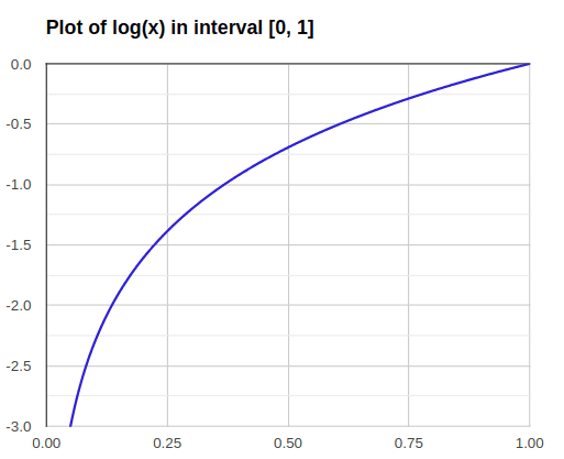
 \hat(y_i) is going to be in [0,1]; thus its logarithm will be between [-inf,0].
For each sample, only the correct class term y_k * log(yhat_k) is going to add to the loss, the rest of the y_i will be zero. If the model is predicting a low probability to the correct class, the log is going to be a large negative number, and the -1 multiplier will make it be a large loss. Vice versa.
Using the new loss, we need to readjust a few derivatives:
dz[L] = Y_hat - Y
The derivative of softmax is:
Y_hat * (1 - Y_hat)
Curiosity: The name softmax comes from contrasting it to what's called a hard max, which would just set a 1 to the largest element and 0 to the rest. Whereas in contrast, a softmax is a more gentle mapping from Z to these probabilities.
Existing frameworks
Deep learning is not about implementing everything from scratch, but about reusing leading existing frameworks.
| Framework | Programming Language | Focus | Deployment | Key Features | Use Cases/Tasks |
|---|---|---|---|---|---|
| Caffe/Caffe2 | C++ | Image/video processing | Production | Modular architecture, speed, image/video focus | Image classification, object detection, image segmentation |
| CNTK | C++/Python | Speech recognition, image recognition, NLP | Production | Computational network toolkit, distributed training | Speech recognition, image recognition, NLP, recommendation systems |
| DL4j | Java | JVM ecosystem, distributed computing | Production | JVM integration, distributed computing | Natural language processing, time series analysis, anomaly detection |
| Keras | Python | Rapid prototyping, high-level API | Production | High-level API, easy to use, modularity | Image recognition, text generation, neural style transfer |
| Lasagne | Python | Theano-based, modular | Research | Theano-based, modular, flexibility | Research, prototyping, building custom architectures |
| MXNet | C++/Python/R/Julia/Scala | Scalability, flexibility, speed | Production | Scalability, hybrid programming, speed | Image classification, object detection, natural language processing, recommendation systems |
| PaddlePaddle | C++/Python | Chinese-dominant, industrial applications | Production | Industrial applications, speed, scalability | Computer vision, natural language processing, recommendation systems, ad optimization |
| TensorFlow | Python/C++ | Large-scale machine learning, distributed computing | Production | Flexibility, scalability, community support | Image recognition, natural language processing, speech recognition, time series analysis |
| Theano | Python | Deep learning research, optimization | Research | Symbolic computation, GPU optimization | Research, prototyping, low-level optimizations |
| Torch/PyTorch | Lua/Python | Flexibility, speed, dynamic computation graph | Research/Production | Dynamic computation graph, speed, flexibility | Computer vision, natural language processing, reinforcement learning |
TensorFlow
The course develops a few concepts of TensorFlow. Here is a sample snippet doing optimization, checkout the programming assignment for more coding examples:
import numpy as np
import tensorflow as tf


coefficients = np.array([[1.], [-10.], [25.]])

x = tf.placeholder(tf.float32, [3, 1])
w = tf.Variable(0, dtype=tf.float32)                 # Creating a variable w
cost = x[0][0]*w**2 + x[1][0]*w + x[2][0]

train = tf.train.GradientDescentOptimizer(0.01).minimize(cost)

init = tf.global_variables_initializer()
session = tf.Session()
session.run(init)
session.run(w)    # Runs the definition of w, if you print this it will print zero
session.run(train, feed_dict={x: coefficients})

print("W after one iteration:", session.run(w))

for i in range(1000):
	session.run(train, feed_dict={x: coefficients})

print("W after 1000 iterations:", session.run(w))- The backward pass is automatically done, you only specify the forward pass.
- A placeholder is a variable that may be assigned a value.
Course 3: Structuring ML Projects
Week 1: ML Strategy
We've discussed many ideas on how to improve a ML model:
- Collect more data.
- Train algorithm longer or use a different optimization algorithm (e.g. Adam).
- Try dropout, L2 regularization.
- Change network architecture (activation functions, # of hidden units, etc.) This course gives strategies to decide in which direction to go.
Orthogonalization
You have to tinker with your ML knobs so that four things happens:
- You fit the training dataset well (e.g. by achieving near HLP on the cost function). If you fail to do this, you can try a more complex architeture, early stopping.
- You fit the validation set well in terms of the cost function. If not, you can try regularization or collecting more training data, early stopping as well.
- You fit the test set well in terms of the cost function. If not, you can try a larger validatin set.
- Your model performs well in the real world. If not, you may need to change the cost function or the validation / val &t est set.
Evaluation metrics
Often it's better to have a single-number evaluation metric for the project before you start it. It could be:
- Accuracy
- F1 score, which combines precision and recall (they don't tell much isolated). This is good for imbalanced datasets. It's the harmonic mean of accuracy and recall.
The harmonic mean is more suitable than the mean when comparing rates. It gives lesss weightage to large values and large weightage to the small values to balance the values correctly.
Say you have Precision = 0.66 Recall = 0.8 => F1 = 0.72 GM = 0.73. Equivalent. Say you have Precision = 0.66 Reall = 0.1 => F1 = 0.17 GM = 0.25. F1 penalizes small values more. F1 better captures the tradeoff between precision and recall.
Sometimes we can define the optimization metric and put constraints to other metrics, because we cannot just find a single metric that captures all:
Maximize F1                           # optimizing metric
subject to running time < 100ms, (..) # satisficing metrics
More generally, if you care about N metrics, you may pick one to be the one you try to do better at, and then you just set thresholds for the others.
Distribution of the test / val / train set
- The val and test set must come from the same distribution. The val set must reflect the data that the model is meant to do well on.
- The val set and the validation metric is defining the overall target. You must make sure to choose a dev and test set that reflect the data where you want to do well on (both now and in the future, foresee future applications!).
- BTW remember it used to be 70/30 or 60/20/20 split; but for larger datasets we use 98/1/1 simil.
Custom dev/test metrics
We may want to customize our metric so that it prioritizes a specific subset of images, e.g. by adding a weight multiplier for certain classes so that misclassifying is penalized more severely.
Comparing to human-level performance (HLP)
We often compare to HLP because it acts as a proxy to the "optimal" classifier (particularly for unstructured data tasks).
After a model reaches HLP often progress slows down a lot, and progress is much harder. The best error possible you can achieve is the Bayes optimal error, there isn't usually much of a gap with HLP. As long as your model is worse than HLP, you can:
- Get labeled data from humans
- Learn from manual error analysis
Say you have the following ML model and context:
| situation 1 | situation 2 | |
|---|---|---|
| Humans | 1% | 7.5% |
| Training error | 8% | 8% |
| Dev Error | 10% | 10% |
| In situation 1, since HLP is just 1%, we need to focus on the bias. The training set is not being fit properly. |
In situation 2, HLP is very close to training error, we need to focus more on variance (improving the dev error).
Thus:
Avoidable bias = Training error - Human (Bayes) error
If this is large, need to reduce bias.
Variance = Dev error - Training error
If this is large, need to reduce variance.
For some problems, DL has surpassed HLP:
- Loan approval
- Product recommendation, online advertising
Humans are far better in natural perception tasks like computer vision and speech recognition. It's harder for machines to surpass human-level performance in natural perception task. But there are already some systems that achieved it.
Improving model performance
1- Look at the difference between HLP and training error (aka avoidable bias). If it is large: a. Train a more complex model or a different architecture b. Train for longer or use a better optimization algorithm c. Find better hyperparameters 2- Look at the difference between the dev/test set and training set error - Variance. If large: a. Get more training data b. Regularization (L2, dropout, data augmentation) c. Use another architecture or hyperparameters.
Week 2: ML Strategy 2
Error analysis
Error analysis: Manually examine mistakes that the model makes. It may give insights into what to do next.
e.g. cat vs dog classification with 10% validation error
- Get 100 mislabelled val images at random
- Count how many are actually dogs
- if 5 out of 100 are dogs, doing better in dogs has the potential to decrease the error to 9.5% at most. It may not be worth working on improvig dogs.
- If 50 out of 100 are dogs, doing better in dogs will decrease the error up to 5%. It's worth working on improving dogs.
You can evaluate multiple error analysis ideas in parallel and choose the best idea. Create a spreadsheet to do that and decide, e.g.:
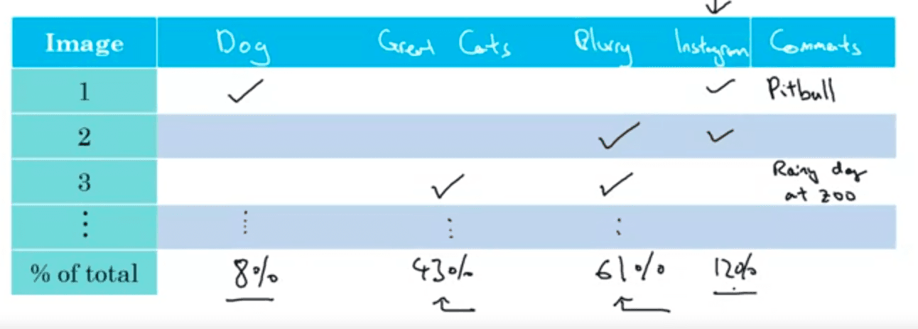
This can help identify a specific subset of images (e.g. blurry cat images) that is worth improving. This quick counting procedure, which you can often do in, at most, small numbers of hours can really help you make much better prioritization decisions, and understand how promising different approaches are to work on.
Cleaning up incorrectly labelled data
DL algorithms are quite robust to random errors in the training set but less robust to systematic errors. We should try to fix these labels if possible.
One possible way is to add a "mislabelled" column in the previous table. That'd give some insight into correction needs.
When correction labels, it is important to:
- Apply the same relabelling criteria in dev and test set
- It's very important to have dev and test sets to come from the same distribution. But it could be OK for a train set to come from slightly other distribution.
- Examine examples that your algorithm got right as well as ones that it got wrong
Practical tips
Build your first system quickly, then iterate:
- Setup dev/test set and metric
- Build initial system quickly
- Use Bias/Variance analysis & Error analysis to prioritize next steps.
Training and testing on different distributions
Sometimes the training set comes from a different distribution than the validation/test sets.
 There are many strategies:
| Strategy | Advantages | Disadvantages |
|---|---|---|
| Shuffle all the data together and extract new train / val / test sets | Distribution of all the sets now is the same | If the dev/test is smaller, their real world distribution will occur less in the dev/test set |
| Take a fraction of the val / test set and move it to training | The distribution that we want to do well is still the target (val/test set) | The train vs val/test distributions are still different, but it's better than the first alternative. |
If train vs val-test distributions are different, the bias/variance analysis using HLP is no longer applicable.
E.g. this setup:
HLP 0% Train error 1% Val error 10%
This may look as a variance problem, but it's actually not clear because of the distribution shift. To solve this we take a subset of the training set called "train-dev set". We do not use it for training, just to evaluate the trained classifier on it. Now:
HLP 0% Train error 1% Train-dev error 9% Dev error 10%
Thus, this is a variance error, because there's no shift in the train-dev set and yet it fails to fit it.
On the other hand
Human error: 0% Train error: 1% Train-dev error: 1.5% Dev error: 10%
This is instead a data mismatch error. Thus, let's define terminology and write steps to deal with mismatched data:
- If
avoidable bias = training error - human level erroris large, use a strategy to reduce bias - If
variance = training-dev error - training erroris large, use a strategy to reduce variance - if
data_mismatch = dev error - train-dev erroris large, this is a data mismatch problem. Use a strategy from the following section - If
test error - dev erroris large, then you need a larger dev set (under the assumption that test and dev sets do come from the same distribution)
Mitigating data mismatch
Try to understand the difference between training and dev/test sets by doing manual error analysis. Then: Option a) Make the training data more similar, maybe using artificial data synthesis techniques (e.g. combine normal audio with car nose to get audio with car noise samples) Opbion b) Collect more training data similar to the dev/test sets.
Transfer learning
Consists of using a model trained for task A and reuse it for task B. In order to do so, the last layer(s) are deleted (along with any incoming weights). Then fine tune the model by adding new last layer(s) and either:
- Keep the weights from the old model A fixed weights and use new (task B specific) data to train the NN and learn the weights of the newly added layers. (suitable for little data of task B)
- Retrain all the weights, allowing modification of the old model A weights as well. (suitable for a larger dataset of task B) Training on task A is called pretraining.
Transfer Learning makes sense if:
- Tasks A and B share the same input X (e.g. imae)
- There is a lot of data for A but relatively less data for B
- Low level features from task A are helpful for learning task B
Multi-task learning
In multi-task learning, you start off simultaneously, trying to have one neural network do several things at the same time. And then each of these tasks helps hopefully all of the other tasks.
Multi-task learning makes sense:
- Training on a set of tasks that could benefit from having shared lower-level features.
- Usually, the amount of data you have for each task is quite similar.
- Can train a big enough network to do well on all the tasks.
End-to-end ML
Some systems have multiple stages to implement. An end-to-end deep learning system implements all these stages with a single NN.
Examples:
Speech recognition
Audio ---> Features --> Phonemes --> Words --> Transcript    # non-end-to-end system
Audio ---------------------------------------> Transcript    # end-to-end deep learning system
Face recognition:
Image ---------------------> Face recognition
Image --> Face detection --> Face recognition
- For some tasks (e.g. speech recognition) end-to-end works better. For other tasks, non-end-to-end works better, even if each step is a separate DL model (face recog).
- End-to-end gives the model more freedom to use the data, e.g. it may not use phonems at all when training speech recognition.
- For end-to-end we need a big dataset.
| end-to-end | non end-to-end | |
|---|---|---|
| pros | does not force the model to reflect human preconceived characteristics or design decisions, lets the NN learn and use whatever statics are in the data. less hand-designing of components and domain knowledge | it may work better in practice when there is not much data available |
| cons | may need a large amount of data, may exclude useful hand-designed components | may use suboptimal components |
| Quiz mistakes: |
Your goal is to detect road signs (stop sign, pedestrian crossing sign, construction ahead sign) and traffic signals (red and green lights) in images. The goal is to recognize which of these objects appear in each image. You plan to use a deep neural network with ReLU units in the hidden layers. For the output layer, which of the following gives you the most appropriate activation function?
Use a Sigmoid on each unit to map it to 0-1. A softmax implies that just one can be present, but in this case all of them could be present.
Course 4
Week 1 - CNNs
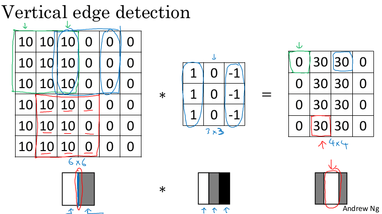
Intuition and edge detection example
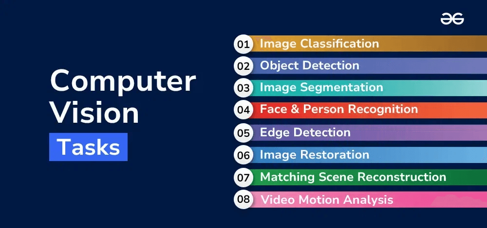
"Computer vision is a field of artificial intelligence (AI) that enables computers and systems to interpret and make decisions based on visual data from the world."
One of the challenges of computer vision tasks is that images are very high dimensional. A 1000 x 1000 image has 3M inputs if we were to use a fully connected neural network. Convolutional layers present an solution to this.
The convolution operation just uses a small filter/kernel (e.g. 3x3), so the number of parameters is way smaller. It's very good at detecting edges, etc ; that subsequent convolutional layers can combine to identify more sophisticated structured.

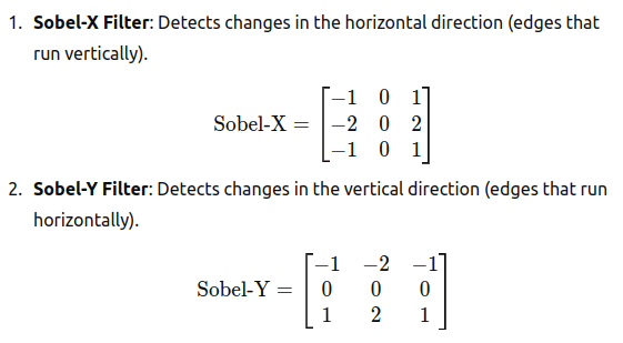
 Other filters are well known, used to detect other type of structures:
- Sobel Filter: Detects changes in the horizontal/vertical direction
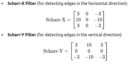
- Scharr Filter: similar to the Sobel filter, but it provides better rotational symmetry and more accurate gradient approximation, especially when detecting edges in images.
 Notes:
- In TensorFlow you will find the function
tf.nn.conv2d. In Keras you will findConv2dfunction.
Padding
- In the last example a
6x6matrix convolved with3x3filter/kernel gives us a4x4matrix. - To give it a general rule, if a matrix
nxnis convolved withfxffilter/kernel give usn-f+1,n-f+1matrix. Thus, the convolution operation shrinks the matrix iff>1
If we don't want to shrink the image of we don't want to lose information from the edges, we can pad the input image by adding zeros around it. The padding amount p is how many columns/rows we insert at the top, bottom, left and right.
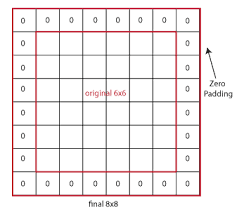 The output size of a convolution with padding
 p is n+2p-f+1,n+2p-f+1
- "same" convolution is the one that produces an output the same size as the input. they use padding
p=(f-1)/2 - "valid" means no padding
Stride
- Add a parameter
sand to govern the stride when sliding the filter. - The output of a filter of size
fand paddingpis(n+2p-f)/s + 1 , (n+2p-f)/s + 1. If fractional, we take the floor.
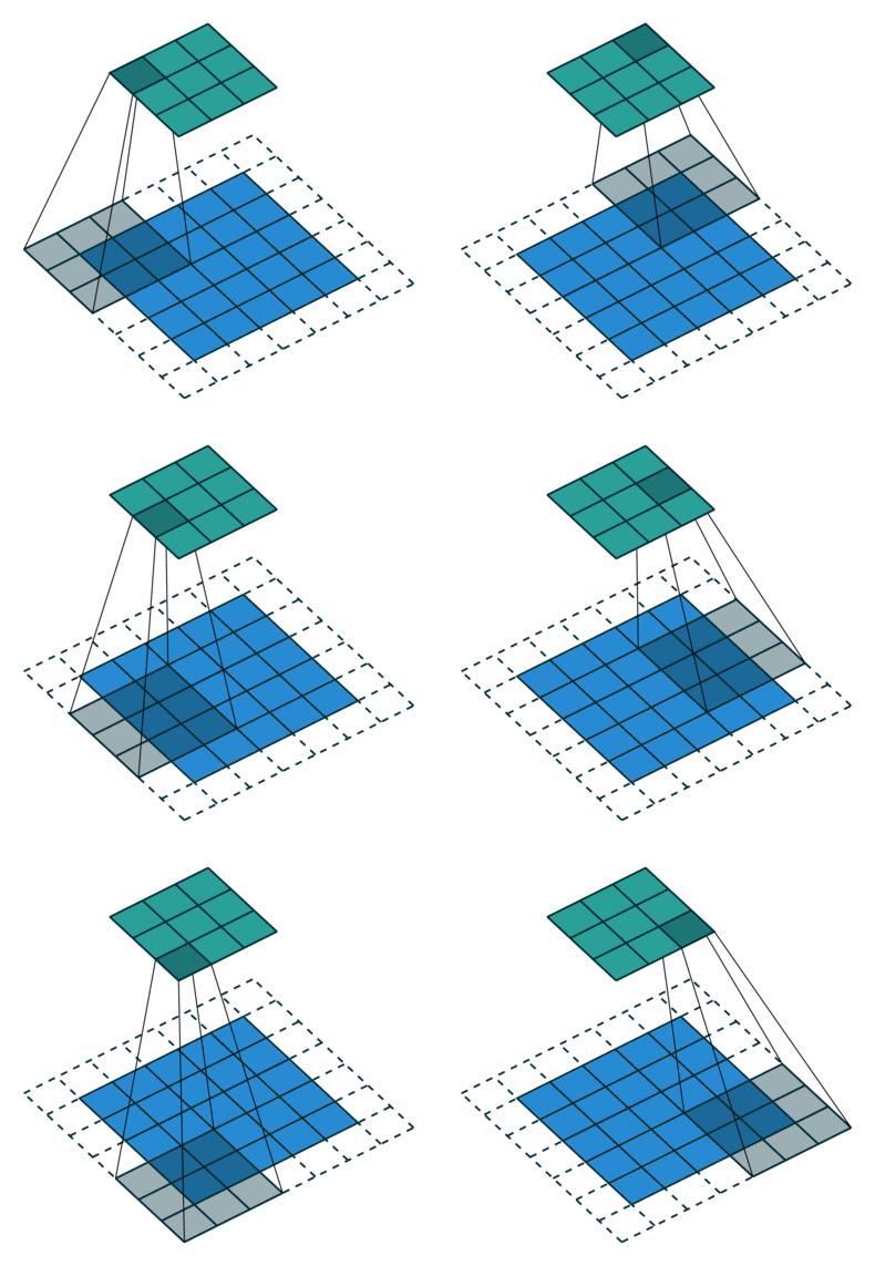
Convolutions over feature maps
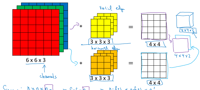
The examples so far dealt with single channel inputs. If we want to convolve a multi-channel input, such as a RGB image, each filter will have to have the same number of channels.
Example:
Input: 6x6x3
Filter: 3x3x3  , p=0, s=1
Result image:  4x4x1
If we want to produce multiple channels, we need to have multiple filters:
Input: 6x6x3
10 filters: 3x3x3  , p=0, s=1
Result image:  4x4x10
If this last example was the layer of a CNN, it would have 10x3x3x3 + 10 parameters (the second term is the bias)
Bias Parameter:
- Each filter has a single bias parameter.
- This bias is added to the result of the convolution for each spatial position after the dot product.
- The bias is shared across all spatial locations for that filter but is not shared across different filters. Each filter has its own bias parameter.
- The bias in a convolutional layer is equivalent to adding a constant value (the bias term) to each element in the output feature map generated by a filter.
Hyperparameters of layer l
f[l] = filter size
p[l] = padding	# Default is zero
s[l] = stride
nc[l] = number of filters

Input:  n[l-1] x n[l-1] x nc[l-1]	Or	 nH[l-1] x nW[l-1] x nc[l-1]
Output: n[l] x n[l] x nc[l]	Or	 nH[l] x nW[l] x nc[l]
Where n[l] = (n[l-1] + 2p[l] - f[l] / s[l]) + 1

Each filter is: f[l] x f[l] x nc[l-1]

Activations: a[l] is nH[l] x nW[l] x nc[l]
		     A[l] is m x nH[l] x nW[l] x nc[l]   # In batch or minbatch training

Weights: f[l] * f[l] * nc[l-1] * nc[l]
bias:  (1, 1, 1, nc[l])
Pooling layer
We reduce spatial resolution by averaging or calculating the max value on each sub-matrix. There's also stride, padding and filter size involved.
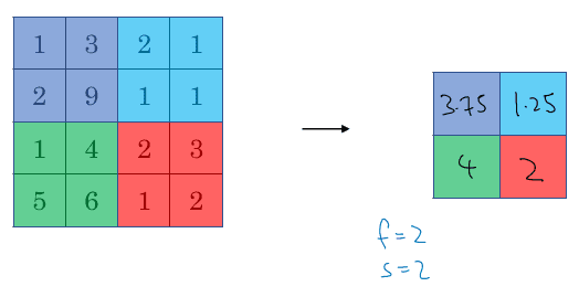
- No learnable parameters
- Max pooling is more popular than avg pooling
- Effect: Summarise information
Simple CNN
Similar to LeNet-5, one of the very first CNNs:
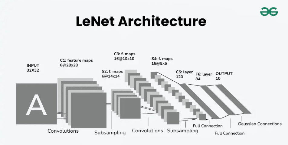
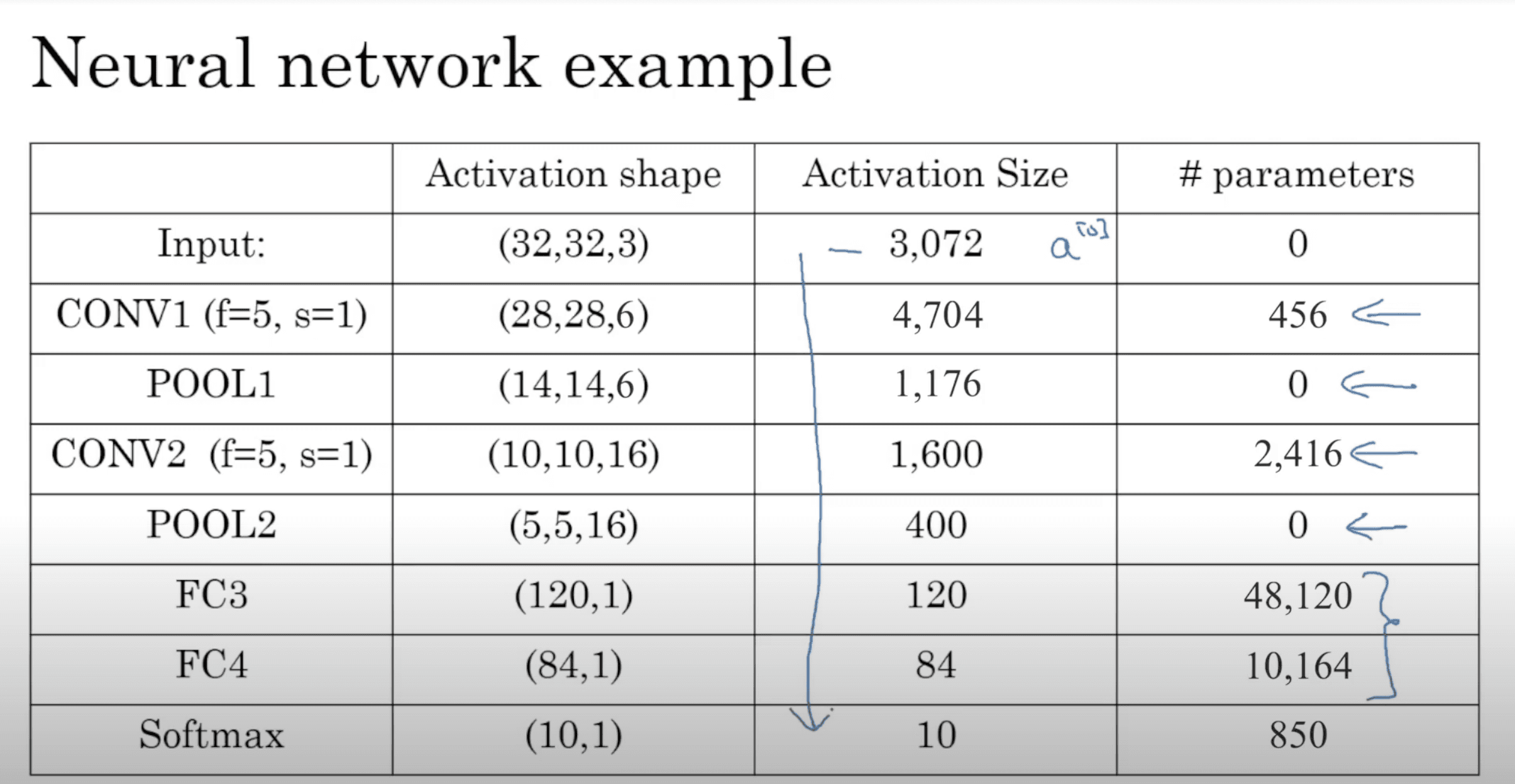 Why does softmax have parameters in this table? something is off.
it is actually referring to the parameters of the FC4 -> Softmax connection.
- Usually the input size decreases over layers while the number of channels increases.
- A CNN usually consists of one or more convolution (Not just one as the shown examples) followed by a pooling.
- Important: "CONV" includes pixel-wise activation function (usually ReLu)
Motivation to use convolutions
- Parameter sharing: A feature detector (such as a vertical edge detector) that’s useful in one part of the image is probably useful in another part of the image.
- Sparsity of connections: In each layer, each output value depends only on a small number of inputs.
- (see my notes on the glossary of layers)
Week 2: CNN Models
CV researchers have spent years studying how to put the layers we have studied (conv2d, poolng, dense)
Classic Architectures I : LeNet-5 (1998)
Used to identify grayscale handwritten digits (32x32x1)

- Used Sigmoid and Tanh back then, nowadays it'd use RELU
Classic Architectures II: AlexNet
Designed for the task of ImageNet with 1k classes:
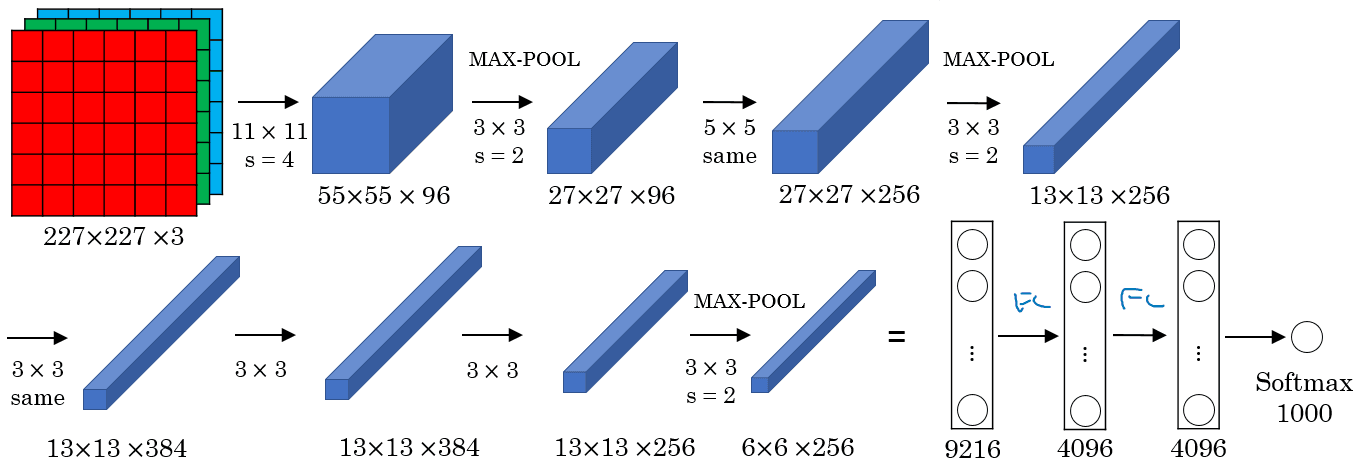
- The ordering of layers is similar to LeNet, but larger
- 60M parameters
- Uses RELU
- This paper was groundbreaking because everyone realised the potential of deep learning
Classic Architectures III: VGG-16
Similar to AlexNet with certain simplifications. All convolutions are 3x3 stride 1; while all poolings are 2x2 with stride 1.
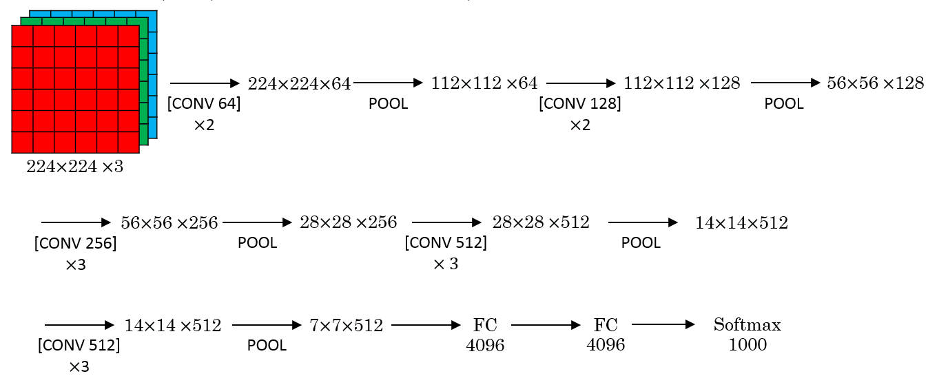
- 138 M parameters, mostly concentrated in the fully connected layers
- Uses 96 MB of memory per image just to do the forward pass - Relatively large, even for today standards.
- Shrinking is done only via pooling
- There are larger versions, e.g. VGG-19.
Residual Networks (ResNets)
ResNets try to address the difficulty of training very deep neural networks (vanishing and exploding gradients), by introducing skip connections. They feed activations from earlier layers to deeper layers, introducing alternative paths for the gradients to flow.
More concretely, ResNet introduces the "Residual Block":
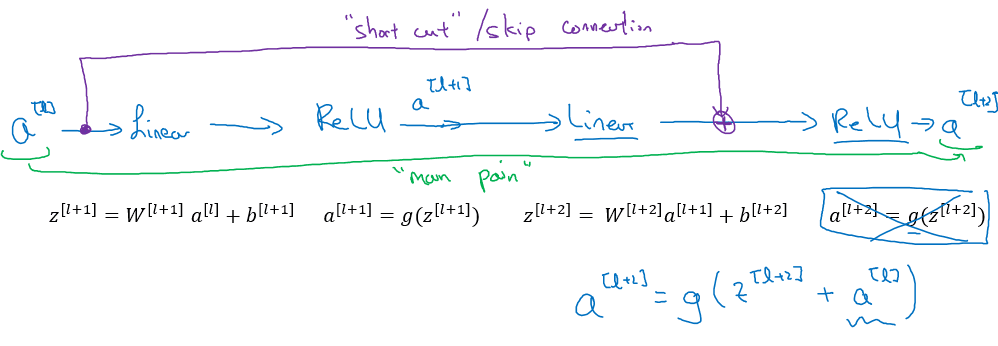 Then, the "Residual Network" architecture consists of many residual blocks stacked together. This allows for deeper networks.
 The heuristic is that deeper networks can do better (provided they have enough data). This is actually problem-dependant. In practice no one goes deeper than hundreds.
Why do residual connectons work?
- Residual connections allow the gradient to flow directly through the network's layers without being diminished. This direct path ensures that the gradient remains sufficiently large, even in very deep networks, thereby alleviating the vanishing gradient problem.
- Residual connections make it easier for the network to learn identity mappings. If a certain layer is not useful, the network can effectively "skip" it by making the residual function zero. This way, the network can easily learn that certain layers should not contribute to the output.
- The network can learn to approximate more complex mappings because it has the flexibility to modify or skip over parts of the input signal while retaining the integrity of the original signal.
ResNet-34
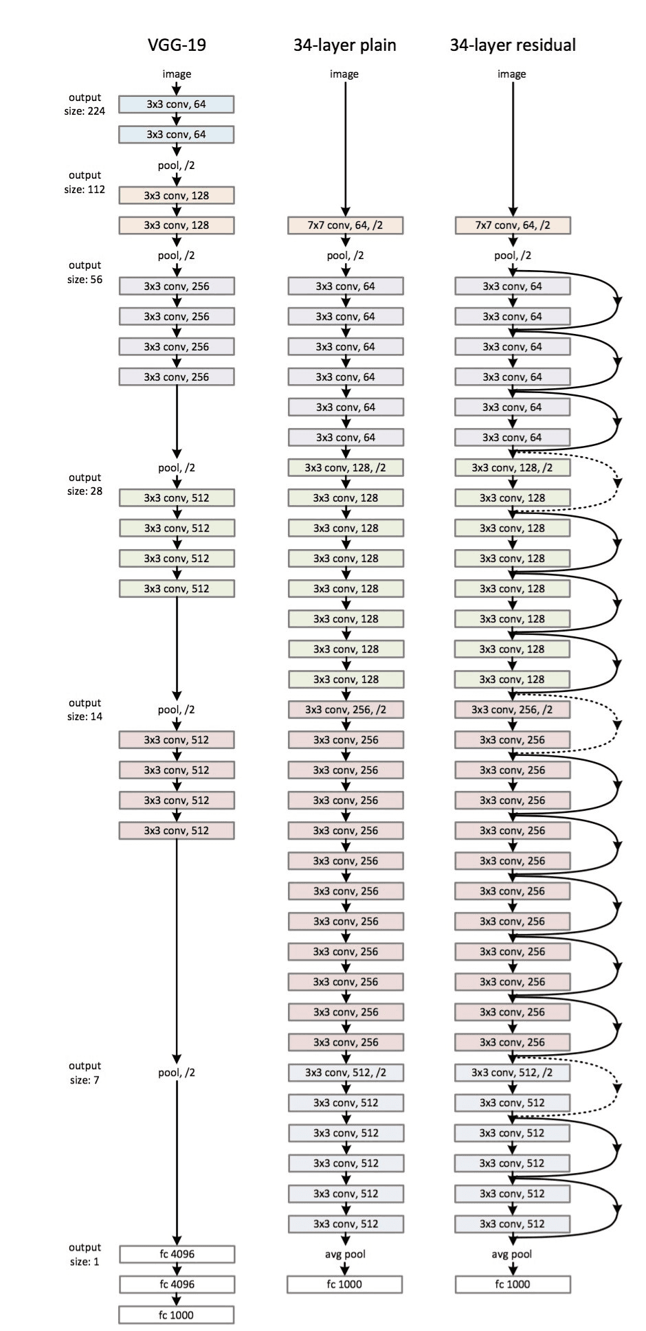 Notes:
- Only uses 3x3 convs
- Spatial resolution keeps being halved, channels doubled
- No FC or dropout
There are two types of ResNet, depending on whether the input/output dimensions are the same or different (dotted lines in the above diagram). The two types of block are:
- Identity block: Dimensions are the same, so we can perform elementwise addition of the activations of layer
lto the pre-activations of later layerl=n.

- Dimension matching: If the dimensions do not match, ResNet uses a projection (typically a 1x1 convolution) to transform the activations from layer
lto the correct shape before performing the addition. The 1x1 conv can easily change the number of output channels to make the number of channels match, whereas the choice of stride can be used to downsample the activations of layerlto make them match.
 here "conv2d" usually is a 1x1 conv.
1x1 Convolutions
- AKA Network in Network , AKA pointwise convolution
- It has been used in a lot of modern CNN implementations,being useful to:
- Shrink or expand the number of channels. We also call this feature transformation.
- Foster inter-channel knowledge exchange
- If the number of output channels is set to be the number of input channels, then the 1x1 conv acts like a non-linearity
- Relu is applied after it, so the non-linearity benefit is always there
Inception Architecture
Motivation
Instead of picking a specific filter size, which can be tricky to optimize, use them all in this Inception module:
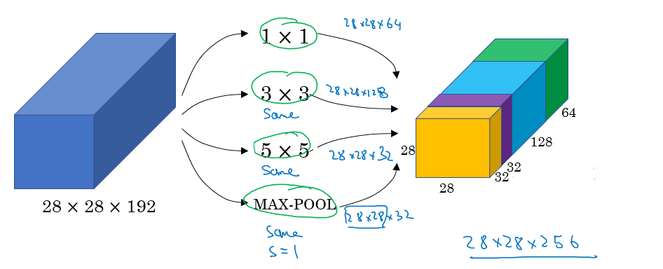 Basically we let the network decide what convolution it wants to use most. However, notice that the module has quite a high computational cost.
Let's consider a 5x5 convolution with same padding and 32 filters applied to a 28x28x192 input. This needs 120M multiplications.
As an alternative, we could first apply a 1x1 convolution that drastically reduces the number of channels, followed by a 5X5 convolution. If the 1x1 convolution has 16 filters, that adds up to 12.4 M multiplications.
The inception module and Inception Network
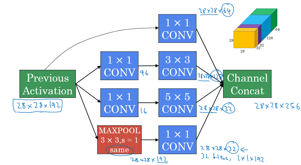 Aka "GoogleNet"
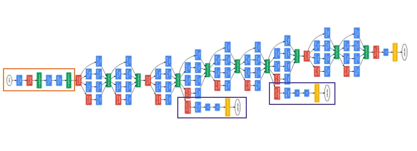
- Concatenated blocks of the Inception module
- There are auxiliary heads
MobileNet
v1
Design to reduce computational costs at deployment, useful for mobile and embedded vision applications.
The key point is the introduction of the depthwise-separable convolution, a more cost-efficient version of the regular 2D convolution.
Say we go from a 6x6x3 volume to 4x4x5 using a 3x3 convolution. This implies a total of 2160 multiplications. There are 5 filter, each one of size 3x3x3
In contrast, a depthwise-separable convolution can achieve the same output shape with significantly fewer computations. Instead of using a full 3D filter, the depthwise convolution applies a single filter of size 3x3x1 to each channel separately. This produces an intermediate volume with the same number of channels as the input. A pointwise convolution (using a 1x1 kernel) then maps this volume to the desired number of output channels. In our example, this approach requires only 672 multiplications—roughly one-third of the computations needed for the standard convolution.
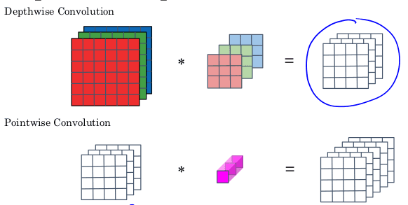 The authors of the paper point out that the cost of a depthwise separable convolution relative to a standard convolution is
 1/num_out_channels + 1/f^2. For f=3 and num_out_channels=5, we get 0.31 the one third improvement we just discussed.
v2
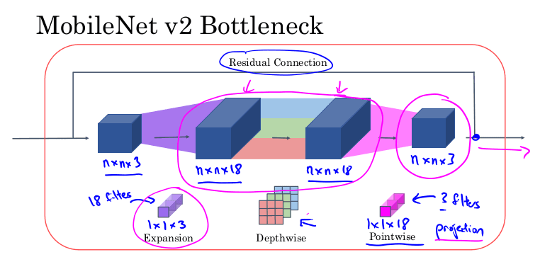
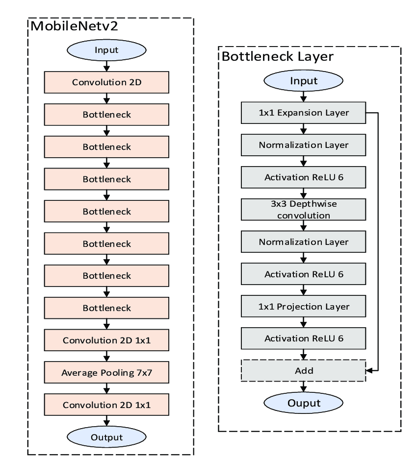
Version two introduces the "Bottleneck module", which expands the number of channels of the input using 1x1 convolutions ; then performs depthwise convolution ; and finally projects back to fewer channels.
EfficientNet
EfficientNet is a family of convolutional neural networks (CNNs) designed by Google researchers to achieve state-of-the-art performance while being computationally efficient. The key innovation of EfficientNet lies in its approach to scaling up neural networks in a balanced and systematic way.
Traditional Scaling: In deep learning, if you want to improve the performance of a CNN, you typically scale it up by making the network wider (more channels), deeper (more layers), or by using higher-resolution input images. However, scaling up in just one of these dimensions often leads to suboptimal performance or unnecessarily high computational costs.
Balanced Scaling: The creators of EfficientNet proposed a new method called compound scaling, where they scale the network’s depth, width, and resolution in a balanced manner. This approach allows for more efficient use of computational resources while improving accuracy.
EfficientNet uses a simple but effective formula (compount scaling) to scale up the network. If you want to scale up the model, you increase the depth, width, and resolution by fixed scaling factors.
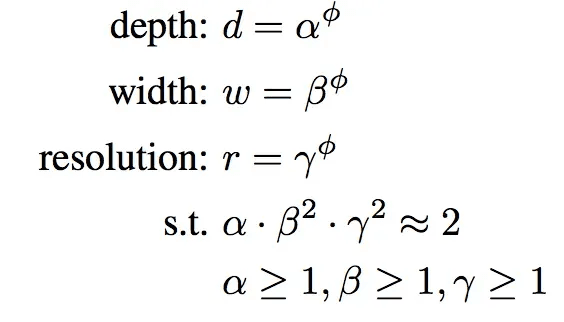
- (phi): This is the compound coefficient. It’s a global scaling factor that controls how much to scale the depth, width, and resolution simultaneously.
- (alpha): This is a constant that controls how much to scale the depth of the network.
- (beta): This is a constant that controls how much to scale the width of the network.
- (gamma): This is a constant that controls how much to scale the resolution of the network
The key idea is that by adjusting phi, you can uniformly scale the network’s depth, width, and resolution to balance the model’s accuracy and efficiency.
| Model | \phi | Depth Scaling (\(\alpha^\phi\)) | Width Scaling (\(\beta^\phi\)) | Resolution Scaling (\(\gamma^\phi\)) | Input Resolution | # of Layers | # of Parameters | FLOPs (Billion) |
|---|---|---|---|---|---|---|---|---|
| EfficientNet-B0 | 0 | 1.0 | 1.0 | 1.0 | 224 x 224 | 82 | 5.3M | 0.39 |
| EfficientNet-B1 | 1 | 1.2 | 1.1 | 1.15 | 240 x 240 | 88 | 7.8M | 0.70 |
| EfficientNet-B2 | 2 | 1.4 | 1.2 | 1.3 | 260 x 260 | 92 | 9.2M | 1.03 |
| EfficientNet-B3 | 3 | 1.8 | 1.4 | 1.35 | 300 x 300 | 98 | 12M | 1.83 |
| EfficientNet-B4 | 4 | 2.2 | 1.4 | 1.4 | 380 x 380 | 114 | 19M | 4.2 |
| EfficientNet-B5 | 5 | 2.6 | 1.6 | 1.6 | 456 x 456 | 126 | 30M | 9.9 |
| EfficientNet-B6 | 6 | 3.1 | 1.8 | 1.8 | 528 x 528 | 138 | 43M | 19.0 |
| EfficientNet-B7 | 7 | 3.6 | 2.0 | 2.0 | 600 x 600 | 150 | 66M | 37.0 |
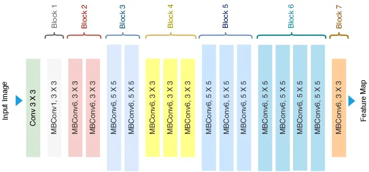 MBConv: Similar to the blocks of MobileNetv2
Transfer Learning
Consists of using the weights of a neural network that has been trained before, using those weights instead of random initialization. This can increase the performance of the NN.
Model pretrained on large datasets like ImageNet, COCO or Pascal take a lot of time and resources to train, and many problems would benefit from reusing the trained models.
Typically the last layer is removed, replaced by a layer suitable for the new task at hand. If there is little data available, make the new network learn only the new layer and freeze the rest of the network (trainable=0). The more data available, the more layers you can unfreeze.
Data Augmentation
Consists of augmenting the data by:
- Mirroring
- Random cropping
- Rotating
- Shearing, warping (geometric transformation)
- Photometric distortion
Takeaways from the Lab - Resnets
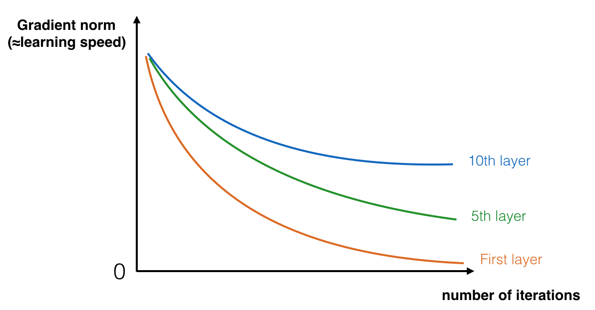 Vanishing Gradient: The magnitude of the gradient decreases significantly for earlier layers as the network trains. We solve this via shortcuts or skip connections.
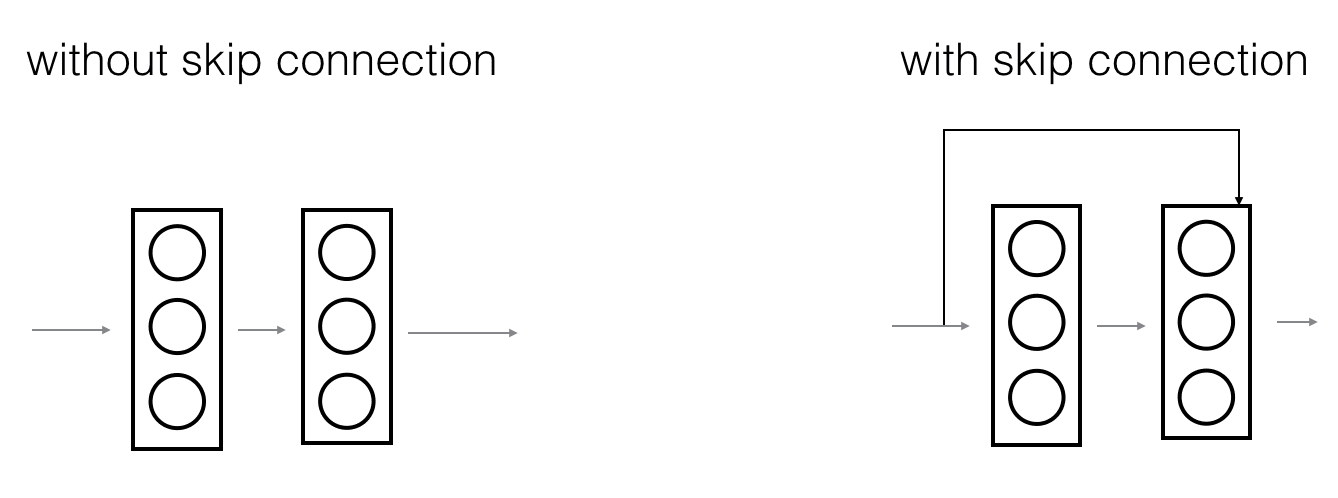 On that note, there is also some evidence that the ease of learning an identity function accounts for ResNets' remarkable performance even more than skip connections help with vanishing gradients.
Two main types of blocks are used in a ResNet, depending mainly on whether the input/output dimensions are the same or different. You are going to implement both of them: the "identity block" and the "convolutional block."
The identity block corresponds to the case where the activations of layer l and l+n have the same dimension. The (+) denotes elementwise addition.

The convolutional block corresponds to the case where the activations don't match, thus we use convolutions to adjust the shape of the shortcut.
 These ID and CONV blocks can be combined to build a large ResNet50 :)

Takeaways from the labs - MobileNetv2
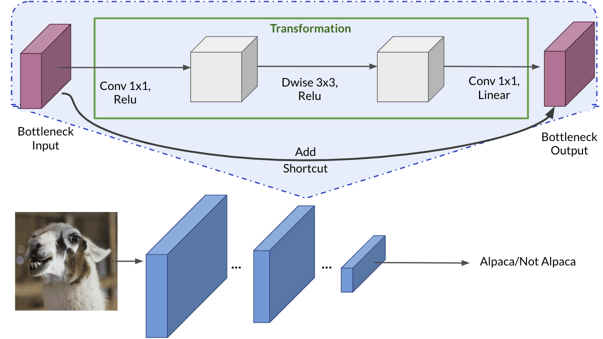 MobileNetV2 uses depthwise separable convolutions as efficient building blocks. Traditional convolutions are often very resource-intensive, and depthwise separable convolutions are able to reduce the number of trainable parameters and operations and also speed up convolutions in two steps:
- The first step calculates an intermediate result by convolving on each of the channels independently. This is the depthwise convolution.
- In the second step, another convolution merges the outputs of the previous step into one. This gets a single result from a single feature at a time, and then is applied to all the filters in the output layer. This is the pointwise convolution.
Each block consists of an inverted residual structure with a bottleneck at each end. These bottlenecks encode the intermediate inputs and outputs in a low dimensional space, and prevent non-linearities from destroying important information. The shortcut connections, which are similar to the ones in traditional residual networks, serve the same purpose of speeding up training and improving predictions. These connections skip over the intermediate convolutions and connect the bottleneck layers.
The lab is very interesting, you load a MobileNetv2 trained on Imagenet, freeze all layers but the last, and instead of returning 1000 classes you now just return 1 (albaca or not albaca image)
Week 3: Object Detection
Object Localization
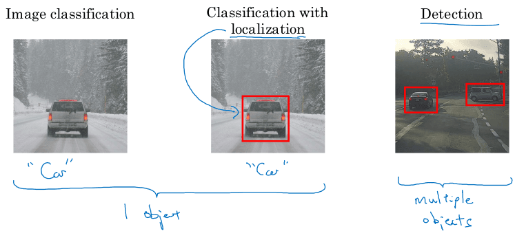
Image classification: predict softmax vector of classes out of an input image. Image classification with localization: Given an image with at most a single object, predict:
y = (p, b_x, b_y, b_w, b_h, c_1, ..., c_k)
Where:
pis whether there is an object or not in the image (0-1)- If
p=1:(b_x,b_y)is the center of the object within the imageb_w,b_hare the width and height of the bounding box relative to the center of the objectc_iare the softmax values for each class
- if
p=0the remaining values don't matter
The loss is:
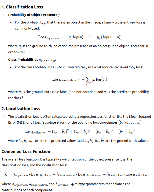
Where we use (check):
- logistic regression loss for
p. - squared error for bounding box coords.
- cross entropy loss for the softmax values.
Auxiliary section: Transforming fully connected layers to convolutional layers
In the next section we will need to replace fully connected layers by convolutional layers. There is a simple, mathematically equivalent way to convert any FC layer to a Conv2D layer.
Say you have a n x n x c_in volume which you flatten into a vector of n*n*c_in and then you apply a FC layer to produce m outputs.
You can write this as a nxn convolution with m filters. Each filter will have c_in channels. This will produce a 1x1xm resulting volume.
Each filter will contain the weights corresponding to a single neuron in the output layer.
The advantage of having a fully convolutional implementation is that you can handle inputs of variable shape, and potentially perform the same computation for different windows
Object detection
In object detection, we may have as many objects as we want on the image, at different scales.
For that purpose, we can train an auxiliary "closely cropped" object localization model on a dataset where all images are neatly cropped to contain mostly the single object in question OR nothing.
Then we may slide a window across the input image, and apply the auxiliary classifier to each crop. We may do this at different window sizes as well.
This can be implemented convolutionally using the very same weights and filters. E.g
Say this is your model trained to predict on cropped images whether there is an object or not and where (image classification with localization):
 You can take the larger image, convolve the same filters (turning the FCs into convolutions to allow for arbitrary input shapes). The result is a feature map that gives, for each crop in your entire input image, the result of the image localization and classification model:
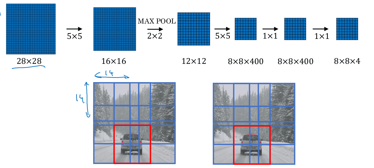
Hopefully the crops that DO contain the car will produce the relevant bounding boxes :)
YOLO agorithm
Let's refine this previous intuition into the popular YOLO (You Only Look Once) object detection model.
We divide the input image into SxS cells (a realistic value would be 19x19, for this silly example it's 3x3). Then the target output for each cell is the same as for image classification with localization. If we have 3 classes, that'd be a 8-valued vector:
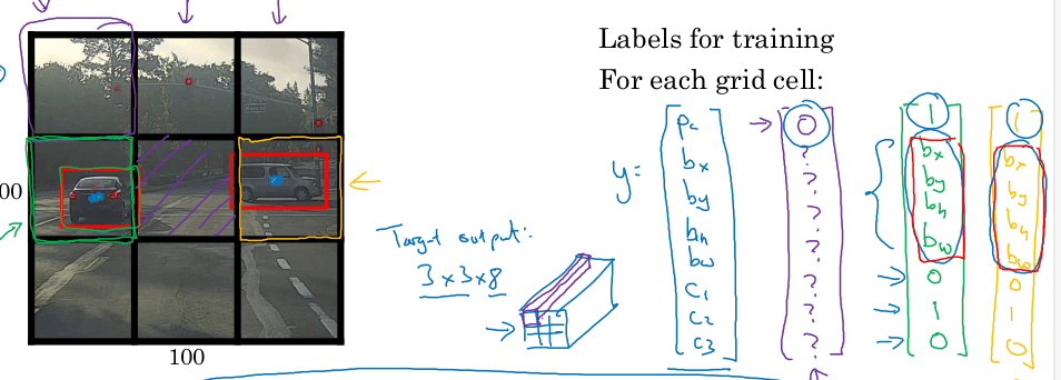
How do we come up with the labels for training? The training set usually describes a list of bounding boxes+class for each image, it doesn't have this concept of "SxS cells" each one predicting 8 values.
So, we build the targets for each cell manually. For each bounding box, we arbitrarily decide that only the cell where the center of the bbox falls is responsible for predicting it. For example, for the green cell, we're going to define a target 8-valued vector that predicts the bbox of the car.
Notice that bbox predicted by a cell can go beyond that cell. That's fine.
If there is no center of a bbox on a given cell, we just place a 0 in the target label and don't care about the rest.
An obvious limitation of this approach is that we are limited to just one object per cell, and if there are two, we cannot represent it. We'll see how to solve that later.
A note on the values of the target vectors that describe the bboxes.
b_xandb_ydescribe the center of the bbox as a fraction of the cell width and height ; so they are values between 0 and 1.b_handb_wcan be larger than 1 and represent the box width and height in "cell size" units.
Non-max suppression
Let's tackle one of the issues of the algorithm as presented so far. The same object can be detected by different cells. Each bbox will have its own center, width, height, class probability, etc.
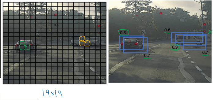 non-max suppression is basically an algorithm to get rid of duplicated bboxes by keeping "the best one" for each object.
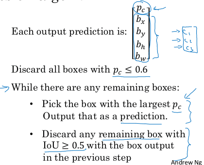
Anchor Boxes
Anchor boxes are an addition to the YOLO algorithm as described above. Instead of predicting just one box per cell, we predict B boxes per cell. Additionally, each of the boxes has a predefined shape or shape ratio, so that each box can "specialize" into different types of boxes. For example, anchor box 1 may be a vertical shape, box 2 may be a horizontal shape. Then, the model is going to predict for each anchor box on each cell modifications to that predefined box to make it better fit the detected object, if any.
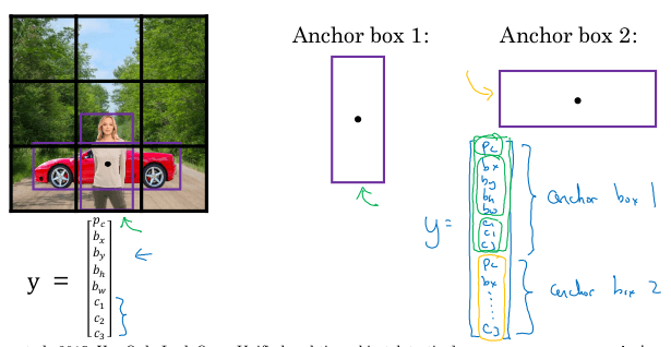 This also allows us to detect multiple objects in a single cells.
It introduces an extra complexity when we build the target ground truth labels to calculate the loss tough. We now need to assign each ground truth bbox not only a cell, but also a specific bbox. We assign the anchor whose IoU with the ground truth box is highest.
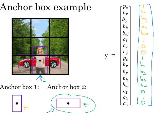
If you have multiple class, perform non-class suppression for each class separately.
Region Proposal algorithms
This is a family or models for object detection that work differently than YOLO. Insted of "just looking once", you process the image at different stages:
1- Propose regions of interest 2-Classify the proposed regions one at a time, producing a label and a bbox
Variants are R-CNN, Fast R-CNN, Faster R-CNN.
- YOLO: Best for speed and real-time applications. It’s fast but less accurate, especially for small objects and crowded scenes.
- Region-Proposal Methods (e.g., Faster R-CNN): Best for accuracy in object detection and localization, especially for small or overlapping objects. However, it's slower and more complex.
Use YOLO when you need speed.
Use region-proposal methods when you need precision.
Semantic Segmentation and U-Nets
The course introduces the task of semantic segmentation, in which we predict the class of each pixel of the input image.
 Unlike image classification and object detection, where we needed to reduce the spatial dimension of the data progressively until we reached the final result; for semantic segmentation we usually need to upsample the spatial dimension back to produce an output whose resolution matches the input.
 To increase spatial resolution we use transposed convolutions:
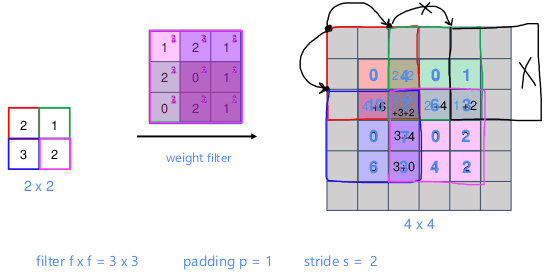
The U-Net architecture makes extensive use of skip connections, convolutions, pooling to downsample and transposed convolutions to upsample:
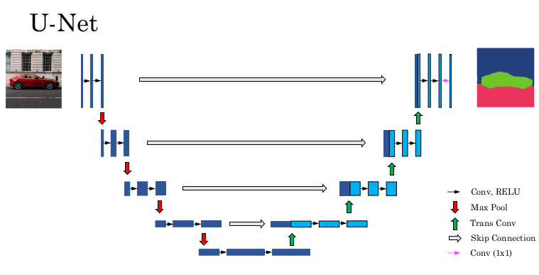 Notice how the skip connections concatenate channels instead of adding like other skip connections we've seen.
Week 5 - Special Applications
Face Recognition
Face Verification: Given an input image and a name/ID, output whether the input image is the claimed person or not. 1:1 Face Recognition: Given a database of K persons, and given an input image, output the ID of the image if it's one of the K persons, else "not recognised". K:1 One-shot learning: Learn from just one example to recognise the person again. More generally:
One-shot learning refers to a model's ability to learn information about a task from only one or a very small number of training examples. Unlike traditional models, which require a large amount of labeled data to achieve high accuracy, one-shot learning aims to generalize from minimal examples, making it particularly useful in cases where gathering large datasets is impractical.
Architectures to solve this issue are:
- Regular image classification, with a softmax and K output neurons. Troublesome, it has to be retrained if the K people change, etc.
- Learning a similarity function:
d(img1, img2) : Degree of difference between images
d(img1,img2) <= tthen "same"d(img1,img2) > tthen "different"
This can be achieved by a siamese network, where a single network is trained to produce an embedding of the objects (faces in this case), and then the embeddings are used to compute the difference:
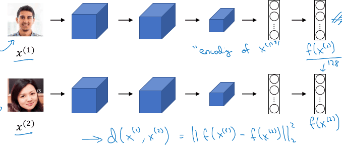 The optimization of this network is achieved via the triplet loss, which aims at getting embeddings that are very distant for different persons and close for the same person.
We pick an anchor image on the dataset, and then a positive image (another sample of the same object) and a negative image (another sample of a different object). Then, for this triplet, we optimize, we define the loss as:

- The alpha is going to encourage the embeddings to not predict something trivial like all embeddings are 0.
- The max is a way to encode that the left side is >= 0
- During training, we pick triplets that are "hard", for instance negative images that are somewhat similar to the anchor image rather than random sampling.
- At inference time we just run the siamese network on two inputs, often one of the output vectors is precomputed, thus forming a baseline against which the other output vector is compared.
A more general case is where the output vector from the twin network is passed through additional network layers implementing non-linear distance metrics:
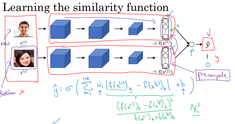
Neural Style Transfer
What are Deep Networks learning?
This section build intuitions necessary to understand neural style transfer better. It basically showcases images from the paper "Visualizing and Understanding Convolutional Networks" by Zeiler et al.
Let's thing of a regular convolutional architecture for image classification such as this one:
 The paper provides a way to understand and visualize what is it that each feature map is learning on each layer, one channel at a time.
For example, let's think about layer 1. The feature map has 96 channels. We can (randomly) pick 9 of those channels, and for each of those channes identify the 9 input patches (from the training images) that maximize the activation of such channel.
The activation of a channel would be the average or the max or the sum of the activations across all spatial locatins.
In the context of training ImageNet, this is what we would come up with:
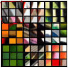 Layer 1: The first filter (channel) seems to detect diagonal edges. In general, earlier layer detect low level features.
The paper provides a method to trace back the activations of each layer to see what patches on the training dataset are activating those feature maps most.
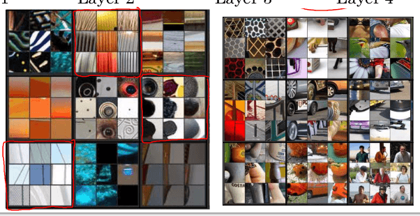 Layer 2 (left) starts to detect more complex patterns and shapes, while layer 3 already increase abstraction further.
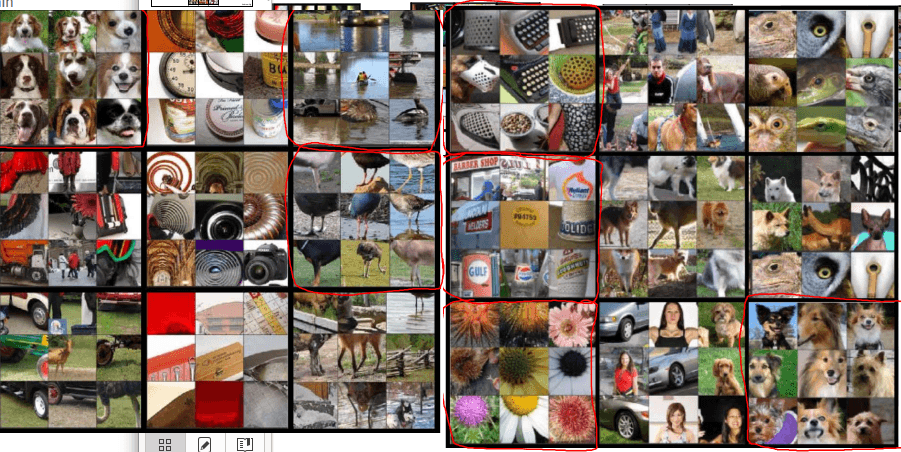 Layers 4 and 5.
The paper is very interesting and provides several visualizations and insights into the CNN black box. It's fascinating.
Neural Style Transfer
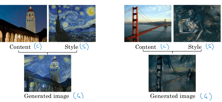
Neural Style Transfer (NST) is a fascinating technique in deep learning that combines the style of one image with the content of another to create a new, blended image. This is done by using a convolutional neural network (CNN), typically a pre-trained model like VGG-19.
- Content Image: This is the image you want to preserve in terms of structure and layout.
- Style Image: This is the image from which you want to extract the artistic style, like the brush strokes or color palette.
- Generated Image: The final image combines the content of the first image with the style of the second.
The cost function to train this network will be:
J(G) = alpha * J_content(C,G) + beta * J_style(C,G)
G will be randomly initialized, although it's often initialized as the content image and noise is applied on top of it, to quicken convergence.
Then, it will be updated using gradient descent and J(G)
G := G - dL/dG J(G)
The content cost function This measures how similar the output image is to the content image by comparing the feature representations at higher layers of the CNN.
- We will pick a hidden layer
lin the VGG to compute the content cost. You will usually get the most visually pleasing results if you choose a layer from somewhere in the middle of the network--neither too shallow nor too deep. This ensures that the network detects both higher-level and lower-level features. - We'll try to ensure that the activations at layer
lare similar when C is the input of the VGG to when G is the input of the VGG. If so, both images have similar content:
J_content(C,G) = 1/2 || a^[l](C) - a^[l](G) ||^2
The style cost function is a bit more complex.
- We will pick a layer
lon the VGG to measure style. We will define style as correlation between activations across channels
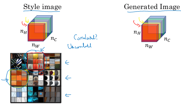
This is, if channels 2 and 4 activations are correlated in the style image S ; we want channel 2 and channel 4 activations to also be correlated in the generated image G.
To this purpose, we will calculate a style matrix G:
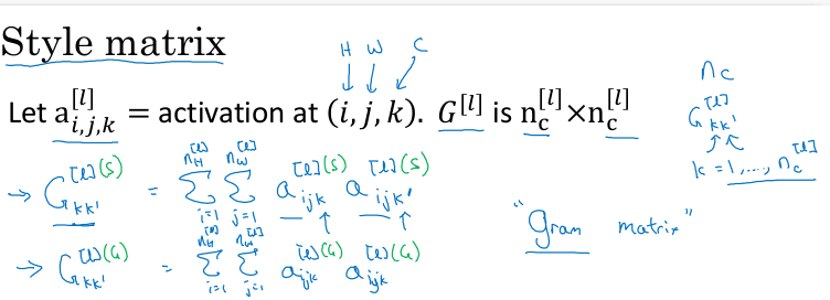
G^[l] is going to measure the correlation for each pair of channels in layer l ; it's the Gram matrix. We can thus try to enforce correlation across channels between the style input S and the generated output G by trying to make the Gram matrixes match:

And actually, as shown in the last equation, for the style cost we calculate the style loss across several layers, not just one as we did for content.
Why is style defined as correlation between channels? because it captures patterns of textures and color distributions that go beyond just spatial structure. The key idea is that style is more about how different features (edges, textures, and patterns) relate to each other across the entire image rather than where exactly they are located.
If we were to define style purely on a pixel-by-pixel basis, we'd lose the abstract patterns that make up style. Instead, using correlations between feature maps lets the model ignore the exact placement of objects (which is more related to content) and focus on more global, perceptual qualities like texture and color schemes.
Course 5: Sequence Models
Week 1: Recurrent Neural Network Model
Basics
Many tasks involve sequential data:
- Speech recognition (sequence to sequence):
- X: wave sequence
- Y: text sequence
- Music generation (one to sequence):
- X: nothing or an integer
- Y: wave sequence
- Sentiment classification (sequence to one):
- X: text sequence
- Y: integer rating from one to five
- DNA sequence analysis (sequence to sequence):
- X: DNA sequence
- Y: DNA Labels
- Machine translation (sequence to sequence):
- X: text sequence (in one language)
- Y: text sequence (in other language)
- Video activity recognition (sequence to one):
- X: video frames
- Y: label (activity)
- Name entity recognition (sequence to sequence):
- X: text sequence
- Y: label sequence
- Can be used by seach engines to index different type of words inside a text.
We can address these problems as supervised learning tasks, provided a labeled training dataset X, Y.
Notation:
X^(i)<t>: the item in position t on the input training sequence i.T_X^(i): Length of the input training sequence i.- Similar notation for the outputs
y.
In tasks that involve text, there are different ways to represent words as fixed-length vectors:
- A predefined corpus of words can be defined (e.g. 10K words), and one-hot encoding can be used to denote each unique word.
- Special tokens like
<UNK>to signal unknown word or<END>to signal the end of the sequence are also employed.
Recurrent Neural Networks
Standard networks (fully connected and CNNs), are unsuitable for sequential data:
- Input and output sequences can have different lengths, but regular networks expect them to have fixed size.
- Feedforward networks process inputs independently of each other, so they cannot account for any relationships between different time steps in a sequence. This limitation prevents the network from learning patterns that unfold over time or remembering prior context
- No concept of "order" in the inputs.
Thus, recurrent neural networks (RNNs) are introduced.
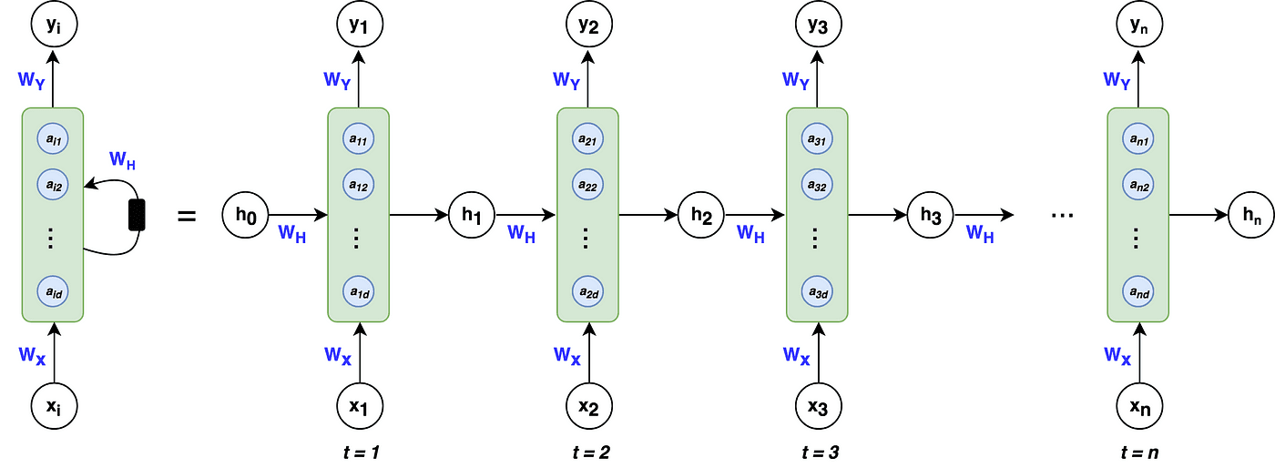
RNNs process input data one time step at a time. At each time step t, the RNN takes the current input x_t and combines it with the hidden state h_{t−1} from the previous time step.
The hidden state h_t serves as the memory of the network, storing information about past inputs. It is updated at each time step using the formula
![]()
The output at each time step y_t can be computed from the hidden state:
![]()
Where W_y is the output weight matrix, c is the bias, and g is an activation function (often softmax or sigmoid).
Note: Andrew uses a instead of h
Remarks:
- We have three sets of learnable weights:
W_h,W_yandW_x. These will be trained via gradient descent. - The same weights are used across all time steps
- activation function
fis usually tanh or ReLU andgdepends on the task, it could be a sigmoid
Dimensions:
d_x: Input dimension. If we are using one-hot encoding with corpus size 10K, thend_x = 10000d_h: Hidden state dimension. Size of the hidden state vectorh_t. This is a hyperparameter.d_y: Output dimension (size of the output vectory_t, fixed)W_xtransforms inputsx_tto hidden statesh_t, thus it has shape(d_h, d_x)W_htransforms the previous state into the current state, thus it's(d_h, d_h)W_ytransforms a hidden state into an output, this it's(d_y,d_h)
RNNs allow for:
- Sequential processing
- Handling variable-length inputs
- capturing temporal dependencies
- take order into account
Backpropagation through time
Backpropagation now is more complicated:
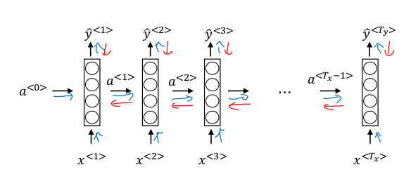
The gradients have to flow back in time.
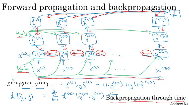 The loss is going to be the addition of the individual loss at each output sequence element. Assuming this is a binary classification task, we could use binary cross entropy loss.
Variations in the architecture
The architecture just presented is suitable for a many-to-many sequence problem. Sometimes we'd only need to output a single value for the entire input sequence (sentiment classification) ; or output a sequence based on a single intput element (music generation).
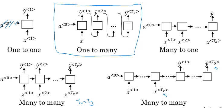
Notice the second many-to-many which has encoder-decoder parts. The encoder encodes the input sequence into one matrix and feed it to the decoder to generate the outputs. Encoder and decoder have different weight matrices.
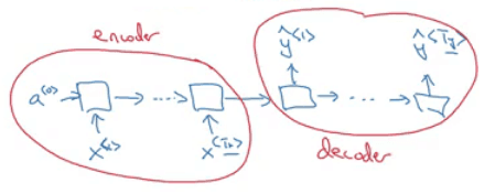
Language Model
A language model is a model that learns the statistical properties of a language and predicts the probability of a sequence of words (or tokens). More specifically, it assigns probabilities to sequences of words in a way that reflects how likely a sequence is to occur in natural language.
This could be useful in speech recognition, to disambiguate between:
- The apple and pair salad -> low probability
- The apple and pear salad -> high(er) probability
How do we build a language model using RNNs?
- Get a training set: A large corpus of target language text.
- Tokenize the training set by defining the vocabulary and applying one-hot encoding to each word.
- Add end of sentence token after each sentence
<EOS>and unknown token for unknown words<UNK> - Each sentence becomes a training sample.
Example, given the sentence "Cats average 15 hours of sleep a day <EOS>", we use this sample to train as follows:
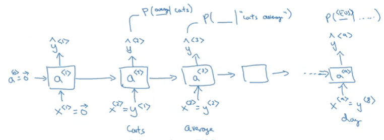 Each
Each y_t being the probability of the next word.
Once this is trained:
- In order to predict the chance of the next word, we feed the sentence to the RNN and get from
y^<t>the hot vector that maximizes the probability. - In order to predict the probability of a sentence, we compute:
p(y^<1>) * p(y^<2> | y^<1> ) * p(y^<3> | y^<1>, y^<2>) * ...
Which is just feeding the sentence into the RNN and multiplying the outputs.
Sampling novel sequences
After a language model is trained, we can sample new sentences by:

- Pass
a^<0> = 0andx^<1> = 0 - Choose a prediction randomly from the distribution
\hat(y)^<1>. This gives us a random beginning for the sequence. - Pass the last predicted word and the hidden state to the RNN. Get a new prediction (presumably the most probable one from the distribution)
- Repeat (3) until the
<EOS>token is predicted
This model was implemented at word-level, it is possible to implement a character-level language model ; where the vocabulary are single characters.
Pros of character level:
- No
<UNK>token, bounded vocabulary, can create any word. Cons: - Sequences are much longer
- Thus, they are bad at capturing long-range dependencies.
- Thus 2, more computationally expensive and harder to train
Remark: The naive RNN is not very good at capturing very long-term dependencies, it quickly forgets what has seen before.
Vanishing and exploding gradients in RNNs
- If sequences are very long, the calculation of the gradients involves many many multiplications. Thus the vanishing gradient problem can arise.
- Exploding gradients can be easily seen when your weight values become
NaN.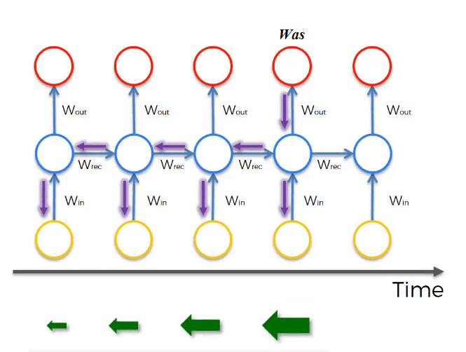
Solve exploding gradients:
- Apply gradient clipping: if your gradient is more than some threshold - re-scale some of your gradient vector so that is not too big. So there are clipped according to some maximum value.
- Truncated backpropagation: Not to update all the weights in the way back. Not optimal. Solve vanishing gradients:
- Weight initialization
- Use LSTM/GRU networks (next)
Gated Recurrent Unit (GRU)
More complex version of a RNN that can help solve vanishing gradients and can remember longer dependencies.
Basic RNN:
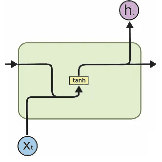
GRU:
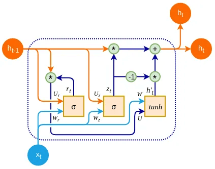
INTUITION Gates are introduced to control what information should be kept, updated or forgotten. The gates help the GRU decide, at each time step, how much of the past information should be passed forward and how much of the current input should be used.
STEP 1: Compute the value of the gates
The candidate activation vector is computed using two gates:
- The reset gate
r_tdetermines how much of the previous hidden state to forget - The update gate
z_tdetermines how much of the candidate activation vector to incorporate into the new hidden state
r_t = sigmoid(W_r * [h_t-1, x_t])
z_t = sigmoid(W_z * [h_t-1, x_t])
The gates use two weight matrices learned during training.
*STEP 2: Compute the candidate activation vector h_t'
GRUs works by computing a candidate activation vector that combines information from the input x_t and the previous hidden state h_{t-1}.
h_t' = tanh(W_h * [r_t * h_t-1, x_t])
Where W_h is also learned during training. The candidate activation vector combines the previous state (after having been reset by the reset gate) and the new input.
STEP 3: Compute the new hidden state
By combining the candidate activation vector with the previous hidden state, weighted by the update gate.
`h_t = (1 - z_t) * h_t-1 + z_t * h_t''
Why this helps
- If the update gate is open (close to 1), the GRU keeps most of the previous information, allowing it to carry forward long-term dependencies.
- If the update gate is closed (close to 0), the GRU focuses more on new inputs, allowing it to update the hidden state with new information.
Because the GRU has this selective memory ability, it can maintain relevant information from many time steps ago
Long Short Term Memory (LSTM)
Another type of recurrent unit, a little more complex than GRU. A third gate is added, called the output gate. This can make LSTM capable or learning more complex patterns, but also more prone to overfitting.
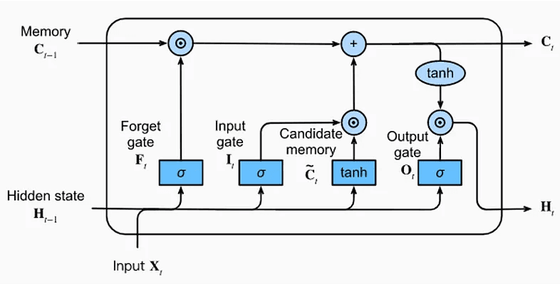
An LSTM unit receives three vectors:
- Two vectors from the LSTM itself at the previous instante: the cell state (C) and the hidden state (H)
- An input vector from the sequence X at time t.
The three gates are information selectors: they create selector vectors with values between zero and one, and near these two extremes (because of sigmoid activation fc).
A selector vector is created to be elementwise multiplied by a vector of the same size. Thus, the selector vector eliminates information in certain positions.
All three gates receive as inputs X_t and H_{t-1}.
The forget gate first decides what information to remove from the cell state.
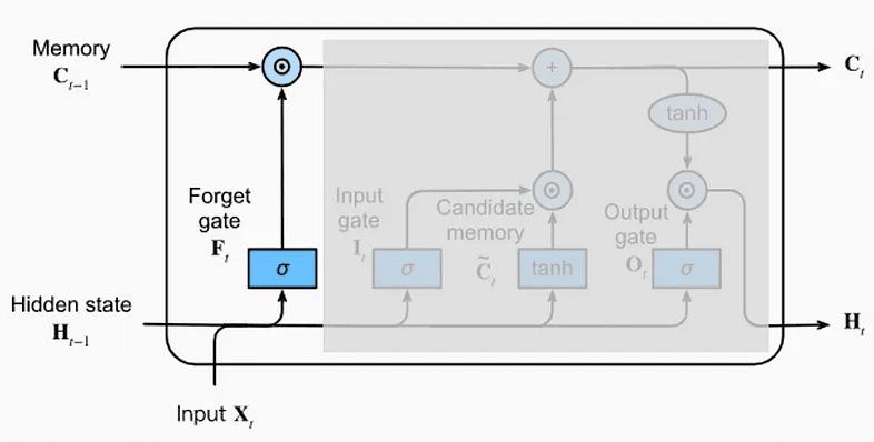
After removing some information from C_{t-1} , we can insert new information.
- The candidate memory generates a candidate vector: a vector of information that is candidate to be added to the cell state.
- The input gate generates a selector vector that is elementwise multiplied with the candidate vector. The result is added to the cell state vector. The resulting cell state vector is passed to the next LSTM unit.
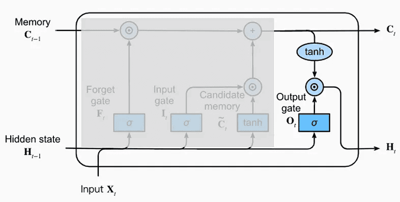
Finally, the output gate is used to generate a hidden state for the LSTM from the cell state.
HIDDEN STATE VS CELL STATE
The cell state is essentially the long term memory of the LSTM. It flows through the sequence with minimal modifications.
The hidden state represents the short term, immediate output of the unit, which is heavily influenced by the current input.
Bidirectional RNN
Bidirectional RNNs are a type of recurrent neural network designed to capture information from both past and future contexts by processing the input sequence in both forward and backward directions. This is particularly useful in tasks where the output depends not only on previous inputs but also on future ones.
The two layers operate independently and have their own hidden states at each time step. After processing the sequence in both directions, the hidden states from both directions are combined (usually by concatenation or summation) to form the final output at each time step.
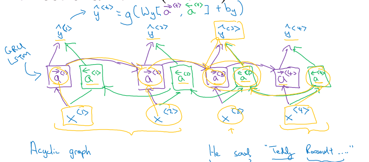 Bidirectional RNNs are ideal for tasks where the entire sequence is available and where both past and future contexts are important. However, if you're dealing with real-time data (like live speech recognition), a unidirectional RNN may be more appropriate because it processes data as it arrives without needing to wait for future inputs.
The blocks here can be any RNN block including the basic RNNs, LSTMs, or GRUs.
Deep RNNs
In some problems its useful to stack some RNN layers to make a deeper network.
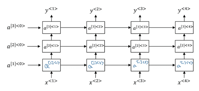 In deep RNN stacking, 3 layers is already considered deep and expensive to train.
In some cases you might see some feed-forward network layers connected after recurrent cells.
| Method | Effective Memory Range |
|---|---|
| Vanilla RNN | ~5 to 10 words |
| GRU | ~10 to 20 words |
| LSTM | ~20 to 50+ words |
| Transformers | ~Unlimited (with attention) |
| Practical assignments: Randomly generate dinosaur names. |
This one provides more insight into how RNNs are actually trained.
- Let's assume that there is a dataset of dinosaur names
- Take each name (which is a sequence of characters) and encode each character into a fixed-length vector
- We are going to train a RNN that predicts the probability distribution of the next letter in the name of a dinosaur.
- From each training dinosaur name, we are going to have a bunch of X,y samples. E.g. from "Triceratops" we get the following training samples:
- Input 0 Output T
- Input: T Output: R
- Input TR Output I
- (...)
- Input TRICERATOPS Output END TOKEN
- We can calculate cross entropy loss of the softmax of the output of the last layer and the one-hot encoding of the correct next letter. E.g. for training sample (3) we assume the ground truth is a probability distribution where letter I has prob 1 and all the rest 0.
After training in many samples, the model learns to distribute these probabilities reasonably.
After we have already trained this mode, at each step the model predicts a probability distribution over characters and we sample from that distribution (instead of picking the most likely character each time). Otherwise, we'd always predict the same names given a starting letter.
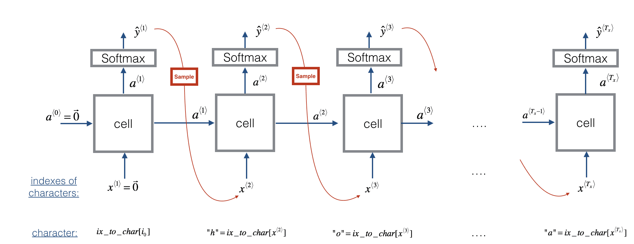
Week 2: NLP and Word Embeddings
Word Embeddings
So far we have defined a fixed-length vocabulary, an represented words as one-hot sparse vectors that identify the word in the vocabulary.
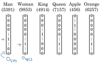
Weaknesses:
- High dimensionality
- Lack of semantic information. This representation does not capture relationship between words. King and queen, related concepts, are represented by entirely different vectors.
- No notion of similarity between words which impairs the ability of the model to generalize learned patterns from one word to the other.
- Mathematically, inner products are always 0 and distances are always the same.
Solution: Learn a featurized representation of each of the words. E.g:
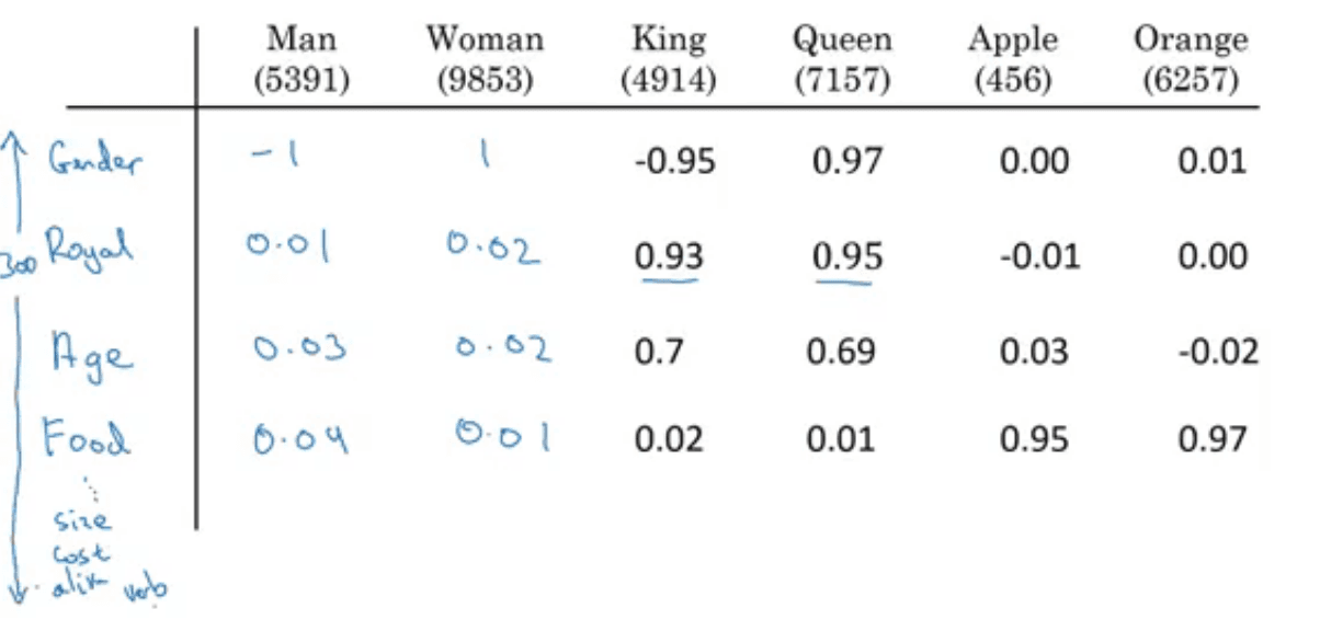
This representation is a word embedding, usually the features do not have such straightforward interpretation, but still are meaningful to establish relationships between different words. Modern word embeddings could use 50 to 1000 features to represent each word.
We can try to visualize this using e.g. t-SNE algorithm to reduce features to 2 dimensions, and the expectation is that related concepts are clustered together:
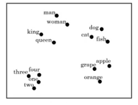
Using word embeddings
Let's consider the task of "named entity recognition"
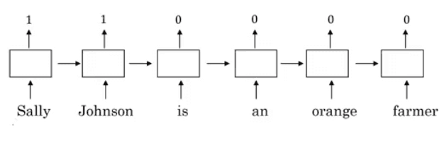 The model should be able to extrapolate from this training sentence and because of the closeness of word embeddings to produce the proper outputs for "Mahmoud Badry is a durian cultivator".
The algorithmos used to learn word embeddings can examine billions of words of unlabeled text and learn the representation from them. It is possible to use learned embeddings from these large corpuses (available for download pretrained) and then fine-tune with a smaller set set of ~100k words.
Properties of word embeddings:
- Lower dimension than one hot encoding, but not sparse
- Similarities between word embeddings are usually calculated via the cosine similarity, which will be large if the verctors are very similar. Euclidian distance could also be used as dissimilarity metric.

A note on this: Cosine similarity:
Cosine Similarity measures the cosine of the angle between two vectors, which means it focuses on the direction or orientation of the vectors, not their magnitude. This is particularly useful when the magnitude of the vectors is not as important as their relative direction. For example, in word embeddings, two words might have different magnitudes (e.g., due to varying frequency in a corpus), but what really matters is how they are related directionally in the embedding space.
Euclidean Distance, on the other hand, measures the absolute distance between two points in the vector space. This can be heavily influenced by the magnitude of the vectors, which might not be desirable when the goal is to assess similarity in terms of direction or semantic meaning rather than size.
This can be used for e.g. analogy reasoning. " man is to woman as king is to _ _ _ _ " We can subtract the respective embeddings:
e_man - e_woman = e_king - e_w
Since we know that the distance between king and queen is approximately the distance between man and woman. To solve analogies like this one, we can calculate argmax_w(e_w, e_king-e_man+e_woman).
-
The word embedding is usually implemented via an embedding matrix (which could be entirely learned). This matrix has one column of each word in the vocabulary
(embedding_size , vocabulary_size)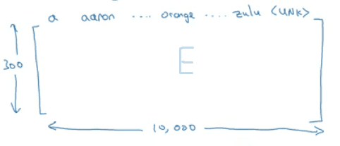 You can basically multiply the one hot embedding of a given word by E and obtain its embedding.
 -
Usually we initialise
Erandomly and then try to learn all the parameters of the matrix.
Word2vec and GloVe
CBOW
Learning algorithms for word embeddings have gone from being more complex to being more simple. Let's follow that order.
Let's consider a model called "bag of words", which is used to learn embeddings. The (self-supervised) task is "next word prediction on a sentence", in other words, a language model.
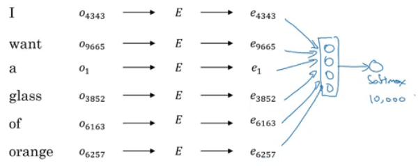
In this setting, we have to optimize:
- E: the embedding matrix
- The weights and biases of the network itself
- Notice that this is not a recurrent neural network. We define a fixed window size (6 here). Meaning that the network takes exactly the last 6 words and predicts the next one.
- This model, built in 2003, produces decent word embeddings.
- The context choice can actually vary:
- We can use a window of words before and after (e.g. 4 previous and next words, and predict the missing word in the middle) this is called continuous bag of words
- Just the last word
- skip gram: Take a single word as input and try to predict the context words around it. It tries to capture the likelihood of surrounding words given a particular word.
To sum up, the language modeling problem poses a ML problem that allows the model to learn good word embeddings.
Skip-gram
Example sentence: "I want a glass of orange juice to go along with my cereal"
- We define a context window, which an integer parameter that determines how many words before and after the target word should be considered. For simplicity, let’s assume a context window size of 2. This means the model will look at 2 words to the left and 2 words to the right of the target word.
- Generate (target, context) pairs. The skip-gram will take each word on the sentence as the target in turn, and generate pairs (target, context). For instance, for the target "glass", it builds the following pairs:
| Context | Target | How far |
|---|---|---|
| glass | orange | -2 |
| of | orange | -1 |
| juice | orange | +1 |
- We train the model as a supervised learning problem where we input the target and try to predict the context.
The network learns to adjust the weights so that, given the input (target word), it can produce outputs that have high similarity to the context words. This is not an easy learning problem because learning within -10/+10 words can become really hard.
If we have a 10k-word vocabulary, the output of the network is a softmax over the 10k words.
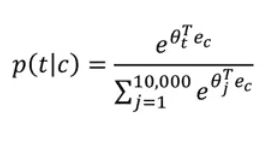 This can be a problem if we have a huge vocabulary like 1M, because it becomes very slow. In this case, we can use a Hierarchical softmax classifier.
Before: A standard softmax layer is used to calculate the probability distribution over the entire vocabulary, which involves a dot product between the input vector and the weight matrix of size V×D (where V is the vocabulary size and D is the embedding dimension) and then normalizing these using a softmax function.
Hierarchical softmax classifier:
- The vocabulary is organized into a binary tree, where each leaf node represents a word in the vocabulary, and each internal node represents a binary decision (left or right child).
- The path from the root of the tree to a leaf node defines a unique sequence of binary decisions that can be interpreted as the prediction process for that word.
- Instead of predicting the probability distribution over all
Vwords directly, the model predicts a series of binary decisions at each node in the tree. - If the tree is balanced, the number of decisions needed to reach a word is approximately
log_2(V) - During training, instead of updating weights for all
Vwords, the model only updates the weights along the path in the binary tree from the root to the target word, making training much faster. - The model is trained to predict the correct sequence of binary decisions leading to the target word.
- The probability of a word is the product of the probabilities of taking the correct path at each internal node leading to that word. The model learns to assign probabilities to these binary decisions during training.
Downsides:
- complexity of implementation
- unbalanced trees
- less accurate estimates
- suboptimal for rare words
In practice, the hierarchical softmax classifier doesn't use a balanced tree. Common words are at the top and less common are at the bottom. Why?
- Computational Efficiency:
- Frequent Words: In natural language, a small number of words are used very frequently (e.g., "the," "is," "and"), while the vast majority of words are rare. By placing these frequent words closer to the root of the tree, the model minimizes the number of decisions (or steps) required to predict these words. Since these words appear so often, reducing the computational cost of predicting them can lead to significant overall efficiency gains.
- Infrequent Words: Rare words, which occur less often, are placed deeper in the tree. While predicting these words requires more steps, the overall impact on computational efficiency is minimized because these predictions are made less frequently.
- Training Efficiency:
- Weight Updates: During training, the model updates the weights along the path from the root to the leaf node corresponding to the target word. For frequent words, shorter paths mean fewer weight updates per prediction, which speeds up training. Since frequent words dominate the training data, this leads to faster overall convergence.
- Less Frequent Words: Although rare words require more updates per prediction, the fact that they appear less frequently in the training data means this does not significantly slow down the overall training process.
Word2vec
Word2Vec is a neural network-based model that learns to represent words in a lower-dimensional space (typically hundreds of dimensions) where words with similar meanings are closer to each other. The key idea behind Word2Vec is to use the context of words to learn these representations.
Word2Vec can be trained using one of the two approaches we just learnt: Continuous Bag of Words (CBOW) or Skip-gram. Both CBOW and Skip-gram aim to create word embeddings that capture semantic relationships between words, but they do so in slightly different ways. CBOW predicts a single target word from its context, while Skip-gram predicts multiple context words from a single target word. Word2Vec can be trained using either the Continuous Bag of Words (CBOW) model or the Skip-gram model, but not both simultaneously.
The choice between CBOW and Skip-gram in Word2Vec often depends on the specific use case, dataset characteristics, and desired outcomes. Here are some general preferences and guidelines:
When to Prefer CBOW:
- Larger Corpora: CBOW is often preferred when you have a large text corpus. It trains faster and can efficiently handle the abundance of context words.
- Frequent Words: If your focus is on predicting common words, CBOW performs well because it averages the context and effectively captures the surrounding information.
- Training Speed: If computational efficiency is crucial, CBOW is typically faster to train than Skip-gram.
When to Prefer Skip-gram:
- Smaller or Noisy Datasets: Skip-gram is preferred when dealing with smaller or noisier datasets, as it can learn better representations for rare words.
- Rare Words: If you want to capture more nuanced relationships and better embeddings for less frequent words, Skip-gram excels because it predicts multiple context words for a single target word.
- Complex Relationships: Skip-gram is generally better at capturing complex relationships and semantic meanings due to its focus on predicting context from a single word.
Negative Sampling
In the original Skip-gram model, the goal is to predict the context words (i.e., words surrounding a target word) for each target word in a sentence. This requires the model to output a probability distribution over the entire vocabulary, which is computationally expensive, especially when dealing with large vocabularies.
Negative sampling is an alternative to the full softmax that significantly reduces the computational complexity. Here's how it works:
Example: "I want a glass of orange juice to go along with my cereal"
| Context | Word | target |
|---|---|---|
| orange | juice | 1 |
| orange | king | 0 |
| orange | book | 0 |
| orange | the | 0 |
| orange | of | 0 |
| We get positive example by using the same skip-grams technique, with a fixed window that goes around. To generate a negative example, we pick a word randomly from the vocabulary. |
We will have a ratio of k negative examples to 1 positive ones in the data we are collecting.
The idea is to train the model to distinguish the true context words (positive samples) from random words (negative samples). Instead of computing a full softmax, the model is trained using a simplified objective function. For a positive pair (w_t, w_c) and a set of negative pairs (w_t, w_n), the objective is to maximize:
 where
where sigma is the sigmoid function.
- The first term maximizes the similarity (dot product) between the target word and its actual context word
- The second term minimizes the similarity between target and negative samples
The model used in this process is a simple neural network with a single hidden layer (essentially a linear model).
Why is the dot product used as a metric of similarity?
- computationally efficient to calculate
- plays nicely with the gradient-based optimization techniques
- The dot product between the target word vector and the context word vector is used to estimate how likely it is that they co-occur. Higher dot products indicate higher similarity, and thus, higher probability.
GloVe word vectors
GloVe (Global Vectors for Word Representation) is another technique to train word embeddings. This is how I understand it:
First, we construct a co-occurrence matrix X, where each entry X_{ij} represents the number of times the word j appears in the context of word i across the entire corpus. The context is typically defined as the words surrounding the target word within a fixed window size. This is a deterministic process.
Then, we are going to train a very very simple model (not a neural network like before). This model is going to take two words (say the ith and jth words of the vocabulary), and it is going to try to predict log(X_{ij}). So the task here is not to predict the missing word, etc ; but to predict the log of the co-occurrence matrix entry. Why the log? Because co-occurrences can vary wildly and a log scale is smoother.
Moreover, the "model" is just going to take the word i and a context word j, calculate its embeddings w_i and c_j via two learnable matrixes W and C respectively, and output w_i^T c_j (their dot product).
The cost function optimized via gradient descent is just a squared error with a weighting factor f(X_ij) which just makes unfrequent combinations weigh less.
![]() Notice that we will use two different embedding matrixes, one for the target word and another for the content word. The final embedding for word
Notice that we will use two different embedding matrixes, one for the target word and another for the content word. The final embedding for word i, having optimized the entire model, is going to be the average of c_i and w_i.
This word embedding will learn vector representations of words by leveraging global co-occurrence statistics from a corpus. The key idea behind GloVe is to learn word vectors such that the relationships between words in the vector space reflect the statistical relationships between words in the corpus.
GloVe aims to capture the ratio of co-occurrence probabilities rather than just the raw co-occurrence counts. This is because these ratios provide meaningful information about word relationships.
Why do this?
- If the dot product of two word embeddings is large, it means that the words iii and jjj are strongly correlated—i.e., they appear together often in the text.
- If the dot product is small, it indicates that the words don’t co-occur frequently or are less related.
For example, words like "king" and "queen" would have a relatively high dot product because they appear in similar contexts, while "king" and "car" would have a much lower dot product since they rarely co-occur in the same contexts.
Notes and examples
- Because word embeddings are very computationally expensive to train, most ML practitioners will load a pre-trained set of embeddings.
- Embeddings are not usually interpretable e.g. an axis is not going to be "gender"
We can then do e.g. sentiment classification using a recurrent architecture and inputing the embeddings:
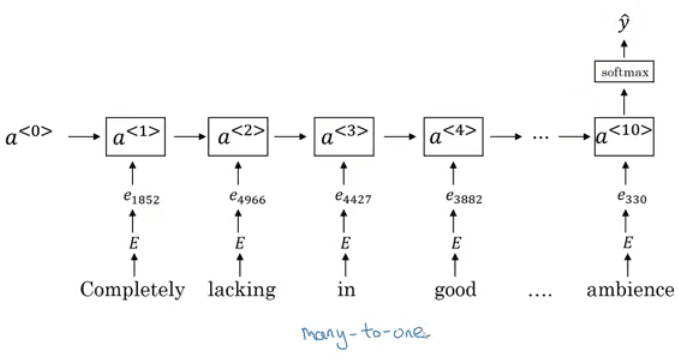
Word embeddings can be "biased" e.g. gender, ethnicity. For instance the analogies "father is to doctor as mother is to nurse" are generated.
We could try to reduce gender bias by intervening the embedings...
"Babysitter and doctor need to be neutral so we project them on non-bias axis with the direction of the bias. The direction of the bias is calculated by averaging the difference between a bunch of pairs of embeddings like (he,she) , (male,female)".
The bottom line:
When learning word embeddings, we create an artificial tasks (such as estimating P(target∣context)). It is okay if we do poorly on this artificial prediction task; the more important by-product of this task is that we learn a useful set of word embeddings.
Week 3: Sequence models and attention mechanism
Sequence models
Models
Let's dive into the task of translating French to English, as concrete example of many-to-many recurrent task. Here's an example:
 We'll work with a recurrent architecture based on RNN (LSTM or GRU included). The left part is the encoder RNN, which takes the input sequence one token at a time. It outputs a vector that encodes the entire input. The right part is the decoder RNN (a different RNN with separate weights), which takes the output of the encoder as the context and generates (one token at a time) the translated sentence.

Notice that the output of the decoder on each step is a softmax across the vocabulary in English. Also instead of starting with an empty/zero context as in vanilla RNN, we pass the output of the encoder as the context of the decoder RNN.
A similar architecture can be used for image captioning, where a CNN encodes an image which is then fed as context input to a RNN.
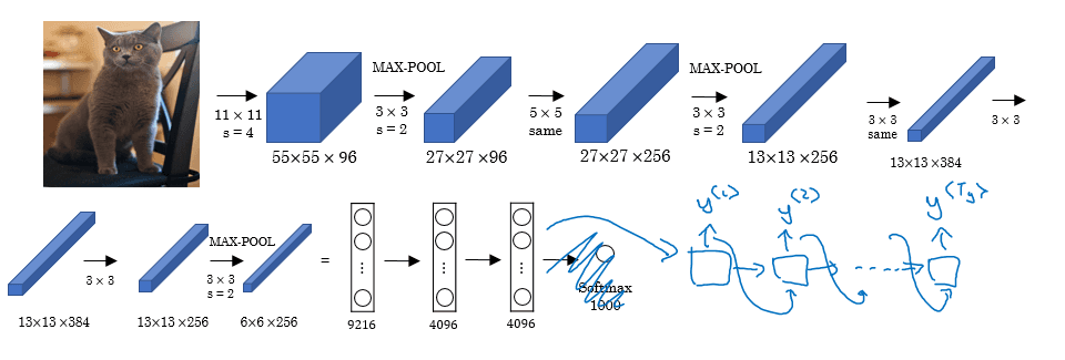
Picking the most likely sentence
Notice that the decoder is going to predict a probability distribution over words in the vocabulary. In the language model setting, when we tried to generate text (e.g. shakespeare poems), we would generate text by sampling from the distribution and feeding it to the network recursively.
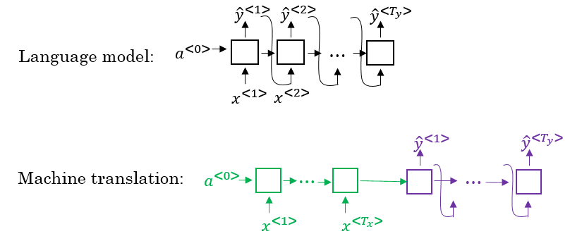
However, for e.g. machine translation, we want the best translation, we don't want to risk sampling something sub optimal:

One may be tempted to go for a greedy approach to pick the final translation:
- Input the French sentence to the encoder, and pass the encoder output as initial context to the decoder
- On each decoder step, pick the most probable (highest softmax) word, add it to the translation so far, and feed it to the RNN recursively.
In practise, this doesn't really work well. E.g:
Suppose that when you are choosing with greedy approach, the first two words were "Jane is", the word that may come after that will be "going" as "going" is the most common word that comes after " is" so the result may look like this: "Jane is going to be visiting Africa in September.". And that isn't the best/optimal solution.
Instead of the greedy approach, we need to get a better solution. The optimal translation would be the one that maximizes the conditional probability (which is the learned softmax):
![]()
This is a huge space of options to explore and it's impossible to find the optimal. Greedy search is a bit of a bad search heuristic, but there is a better alternative: beam search.
Beam search helps approximate the most likely translation by keeping track of multiple hypotheses at each time step. If you generate the translation word by word using only the highest-probability word at each time step (greedy search), the model might miss better overall sequences because some of the best translations may involve words with lower probabilities at earlier time steps.
Beam search mitigates this by exploring multiple possibilities in parallel, keeping track of the top k most likely sequences (where k is the beam width, a hyperparameter).
- Initialization:
- Start with the encoded sentence from the encoder.
- The first word of the output sequence is typically a special token, such as
<start>. - At the first time step, the decoder outputs a probability distribution over the target vocabulary using softmax.
- Beam Expansion:
- Instead of choosing just the most probable word (as in greedy search), beam search selects the k most probable words (beam width k).
- Each of these k words is considered as the start of a possible translation. These words become separate hypotheses.
- Recursion:
- For each of these k hypotheses, the decoder generates the next word’s probability distribution (softmax).
- For each hypothesis, you compute the probabilities of continuing the sentence with each word in the vocabulary.
- Now, you have k hypotheses, each with a full vocabulary of possible next words. But you only keep the k best sequences across all hypotheses (based on their cumulative probabilities).
- This process repeats for each time step until an end condition is met (like an
<end>token or a maximum sequence length).
- Cumulative Probability:
- Beam search tracks the overall sequence probability, which is the product of the probabilities of the chosen words at each step.
- Since probabilities are between 0 and 1, their product decreases exponentially. To avoid numerical underflow, log probabilities are typically used. So, instead of multiplying probabilities, the log probabilities are summed.
In industry standards, perhaps k=10 is a normal result ; in academia they may use k ~ 1000 when trying to squeeze the maximum performance possilble. k=1 is greedy search.
Length optimization
Length optimization: Recall that the cumulative probability that we keep and try to optimize is the product of the conditional probability of each word:

P(y<1> | x) * P(y<2> | x, y<1>) * ... * P(y<t> | x, y<y(t-1)>)
Since probabilities are almost always lower than 1, this makes longer sequence have smaller probabilities and thus (1) cause numerical instability (2) benefits shorter translations.
To solve (1) we sum the logs, and optimize the log probabilties.

To solve (2) we normalize by the number of elements in the sequence (powered to a hyperparameter that actually governs how much we normalize... people use 0.7)

To optimize k (called B sometimes) we may look into the errors:
- Look at a bunch of samples that were mistranslated
- Calculate the cumulative probability of the translation and of the ground truth.
- If the probability of the beam-search approximation is way smaller than the probability of the ground truth, they there is a search issue, and perhaps increasing B is a good thing.
- otherwise, the RNN is at fault
BLEU Score
The BLEU (Bilingual Evaluation Understudy) score is a metric used to evaluate the quality of machine-translated text by comparing it to one or more reference translations. It’s widely used in machine translation to assess how close the generated translations are to human translations, since there may be many valid translations.
An n-gram is a contiguous sequence of words in a sentence. For example:
- 1-gram (unigram): "the"
- 2-gram (bigram): "the dog"
- 3-gram (trigram): "the dog sleeps"
- BLEU typically considers up to 4-grams (unigrams, bigrams, trigrams, and 4-grams). BLEU measures the overlap of n-grams between the machine translation and the reference translations.
BLEU computes precision for n-grams, which is the proportion of n-grams in the machine translation that match n-grams in the reference translation(s).
E.g: reference translation: "The cat is on the mat" machine translation: "The cat is mat"
- Unigram precision: The unigrams in the machine translation are "The", "cat", "is", and "mat". These words also appear in the reference translation. So, the unigram precision is 4/4=1
- Bigram precision: The bigrams in the machine translation are "The cat", "cat is", and "is mat". Only "The cat" and "cat is" appear in the reference, so the bigram precision is 2/3=0.67.
- Trigram precision: "The cat is" and "cat is mat" ; thus 0.5
- 4-gram precision: There is a single 4-gram, which is not in the reference. thus, 0/1 = 0.
Importantly, BLEU uses modified precision to avoid rewarding the model for simply repeating words many times. It caps the count of each n-gram by the maximum number of times it appears in the reference.
E.g. if the prediction is "the the the the", the unigram precision is 1/4 insead of 4/4.
BLEU also implements a BP penalty (brevity penalty) to penalize too short sentences:

Putting it all together, the final BLEU score is the product of the geometric mean of the n-gram precisions, times the brevity penalty.

BLEU = BP * P_n
Strengths:
- Simple and fast: BLEU is easy to compute and widely accepted.
- Works well with large datasets: It correlates well with human judgments when comparing many translations. Weaknesses:
- No consideration of meaning: BLEU focuses purely on matching words and n-grams, without considering whether the translation is grammatically correct or preserves meaning.
- No reward for fluency: A translation can score highly even if it's awkward or unnatural, as long as it has good n-gram matches.
- Shortcomings for individual sentences: BLEU was designed to work well on corpora (large datasets), so its usefulness for evaluating individual sentences can be limited.
Motivating the next section
- If you had to translate a book's paragraph from French to English, you would not read the whole paragraph, then close the book and translate.
- Even during the translation process, you would read/re-read and focus on the parts of the French paragraph corresponding to the parts of the English you are writing down.
- The attention mechanism tells a Neural Machine Translation model where it should pay attention to at any step
Attention model intuition
The attention mechanism was indeed introduced in the context of machine translation, specifically to address some key limitations of the basic sequence-to-sequence (Seq2Seq) models using RNNs (LSTMs/GRUs).
Problem with Basic RNN (Seq2Seq) Model:
In the basic Seq2Seq model:
- The encoder reads an input sentence (e.g., in French) and encodes it into a fixed-size context vector (also called the hidden state), which is passed to the decoder.
- The decoder then generates the translated sentence (e.g., in English) word by word based on this context vector.
The context vector is a fixed-size summary of the entire input sentence, no matter how long the sentence is. This can lead to two key issues: information bottleneck and context loss over long sequences.
How the Attention Mechanism Helps
The attention mechanism was introduced to overcome these limitations by allowing the decoder to focus on different parts of the input sentence at each decoding step. Instead of relying on a single fixed context vector, attention gives the model the ability to access all hidden states of the encoder dynamically.
Here’s how attention helps:
- At each step of the decoder’s generation process, instead of using a single fixed context vector, the decoder can attend to specific words in the input sentence, using a weighted combination of all the encoder's hidden states.
- The model learns to decide which parts of the input are most relevant to the current decoding step.
How the Attention Mechanism Works:
-
Encoding:
- The input sentence
X=(x1,x2,…,xn)is passed through the encoder (an RNN/LSTM/GRU). - At each time step, the encoder generates a hidden state
h_t, which is a representation of the input word at that time step, capturing both the current input word and the context of previous words. - Instead of collapsing all these hidden states into a single vector, we keep all hidden states, one for each word in the input.
- The input sentence
-
Decoding with Attention:
- At each step
tof decoding, the decoder generates a hidden states_t (its internal representation at time stept, based on the words generated so far). - The attention mechanism then computes attention scores for each encoder hidden state
h_i, determining how much attention to give to each input word. - The attention score
e_{t,i} between the decoder hidden states_t and the encoder hidden stateh_i is calculated, typically using a similarity function such as dot product, general linear transformation, or learned neural network function (e.g., a small feed-forward neural network): e stands for energies
 - These scores are then normalized to form attention weights
\alpha_{t,i}using the softmax function:
- The attention weights
\alpha_{t,i} represent the importance of each encoder hidden stateh_i for the current decoding stept.
- At each step
-
Context Vector:
- Using the attention weights, the model computes a context vector for the current decoding step. The context vector
c_t is a weighted sum of the encoder hidden statesh1,h2,…,hn:
- This context vector
c_t contains information about the parts of the input sentence most relevant to generating the current output word.
- Using the attention weights, the model computes a context vector for the current decoding step. The context vector
-
Generating the Output Word:
- The decoder uses both its current hidden state
s_t and the context vector ctc_tct to predict the next word in the output sequence:
- This step generates the probability distribution over the target vocabulary, from which the next word is chosen.
- The decoder uses both its current hidden state
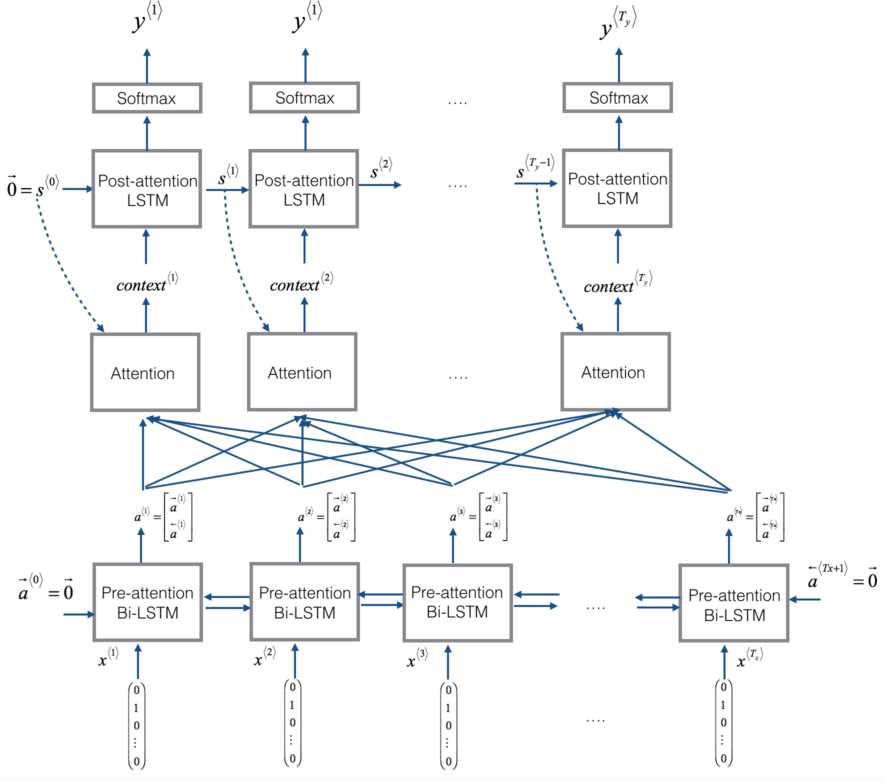
Here we can zoom into what a single "Attention" block is doing:
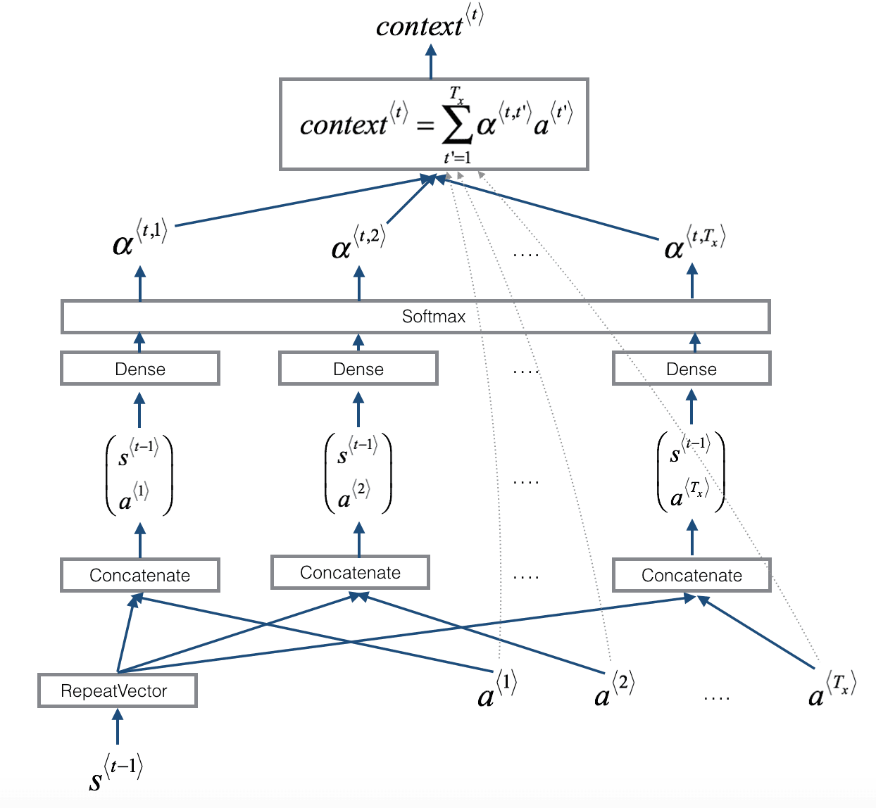
To sum up: When generating output token t, we do it by combining all hidden states from the encoder, weighed by attention coefficients. Then we pass on a context. Notice that the encoder may be a bidirectional RNN.
Notes:
- There are two separate LSTMs in the previous model: pre-attention (encoder) and post-attention (decoder).
- If we use LSTM, remember that it has both a hidden state and a cell state.
- There are variants where the post-attention LSTM at time t' only takes the hidden state
s_tand the cell statec_t, but not the prediction at the previous time-step; this may be suitable for applications where there isn't a strong dependency between previous character and next character (unlike language translation)
 simplified view
The complexity of attention
The attention mechanism described above involves computing scores between the current decoder hidden state and every encoder hidden state.
For each output word t (where the length of the target sequence is m), we calculate the score for n words in the input sequence. Thus, m x n operations. If m and n have similar lengths, this means that the computational cost is O(n^2)
This means the computational cost grows quadratically as the sequence gets longer
Visualising attention weights
 The image shows which words in the English sentence are most important for predicting each word in the French sentence according to the attention mechanism.
Speech recognition
A clip of audio is just a sequence of numbers. e.g. a 10 second audio clip is represented by 441000 numbers.
You can build an accurate speech recognition system using the attention model that we have descried in the previous section. One of the methods that seem to work well is CTC cost "Connectionist temporal classification".
Notice, that the number of inputs and number of outputs are the same here, but in speech recognition problem input X tends to be a lot larger than output Y.

The CTC cost function allows the RNN to output something like this:
ttt_h_eee<SPC>___<SPC>qqq___ (from a clip saying "the q") where
_is the blank caracter<SPC>is the space character- A basic rule is to collapse repeated characters not separated by blank
There is an interesting assignment where we predict 1 in a sound clip if the word "activate" has just been said. Similar to what an alexa would do when someone says alexa.
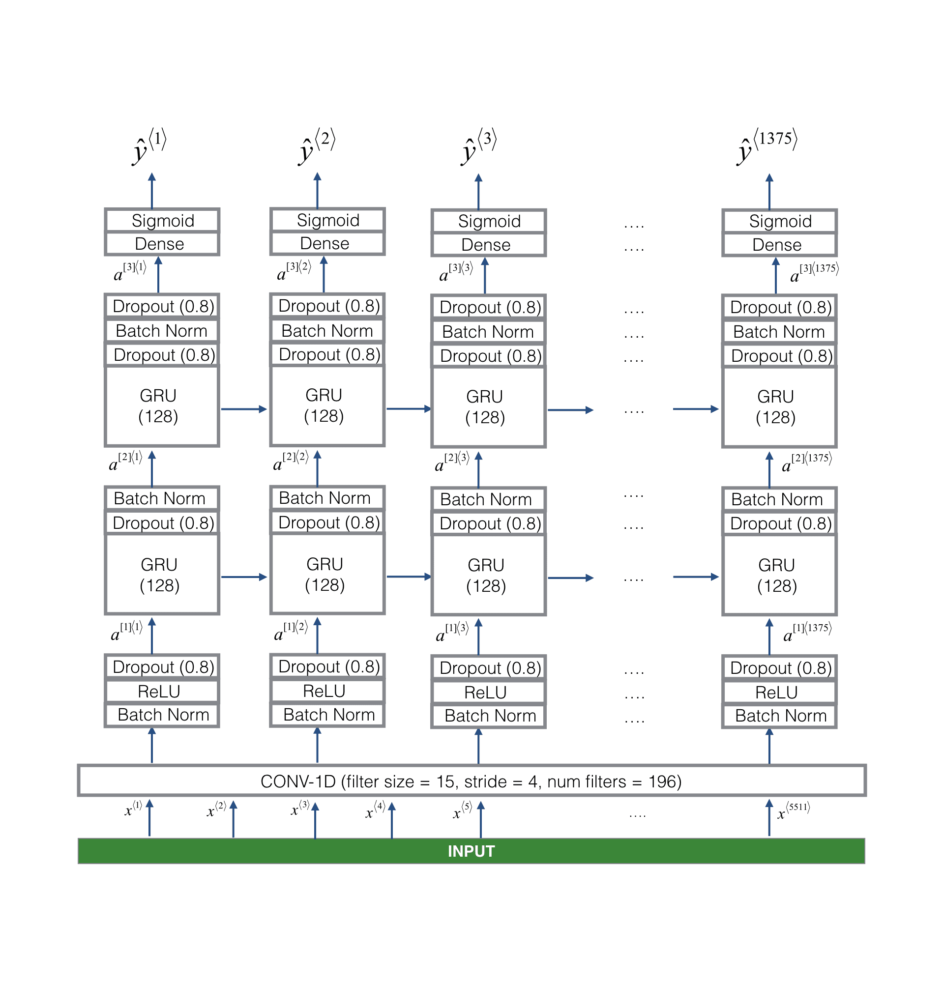
Week 4: Transformers
Self-Attention
Intuition: We have studied architectures that are able to process sequential data, but they have the disadvantage that they have to process each input token one at a time.
Transformers overcome this limitation by processing the entire input at once. For each element in the input sequence x^<i>, the self-attention mechanism is going to calculate another representation of that element A^<i> by looking at the surrounding elements of the sequence and producing an "attention-based" representation.
E.g. for l'Afrique in the following sentence, it will produce a "contextualized representation" of the word. It actually does this in parallel for all words.

The actual calculation of A^<i> bears some resemblance to the attention mechanism we studied before, in the sense that a softmax is calculated.

However, there are a lot of new terms. For instance, in order to calculate the self-attention representation A^<3> of l'Afrique, we proceed as follows:
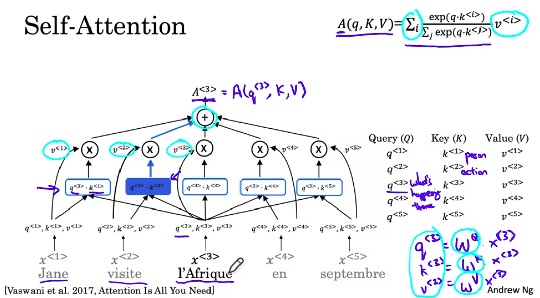
(1) for each input element Calculate three vectors q<3>, k<3> and v<3> (query, key and value) using a learned projection W^Q, W^K, W^V.
- The query: "What's happening there?" (in
l'Afrique) - The key tells us how good an answer each other word is
q<3> . k<1>: How good an answer to the question word 1 isq<3> . k<2>: How good an answer to the question word 2 is.- Each dot product tells us how much relevant as a context each other word is. They are called attention scores.
(2) We will calculate a softmax over all the q<3> . k multiplications. The result is a probability distribution, since all resulting attention weights add up to 1. Remark: They are single scalar values associated with each sequence element.
- WHY A SOFTMAX? The scores might not be bounded, leading to potential instabilities during training..
(3) We calculate a weighted sum of all the values using the output of the softmax as coefficients.
We can actually compute everything at once:

d_kis a scale to the dot product to prevent convergence issues
Multi-Head Self-Attention
We will have N blocks of self attention running in parallell.
Given an input X, each of the N heads will calculate its own K_h, Q_h, V_h using its own learnable matrixes.
The output of each head will be a tensor of the same dimensionality than X.

Since we have n heads, we'll have n attention outputs that will be concatenated along the feature dimension.
Concat(head1,head2,…,headH)
Finally, a learnable weight matrix W^O is used to combine information from all heads and project it back into the original dimensional space (same shape as X)
Intuition: Each head can focus on different parts of the sequence or capture different relationships between words or tokens.
Practical tips: The number of heads usually ranges between 8 (original transformer) and 24 (GPT-3).
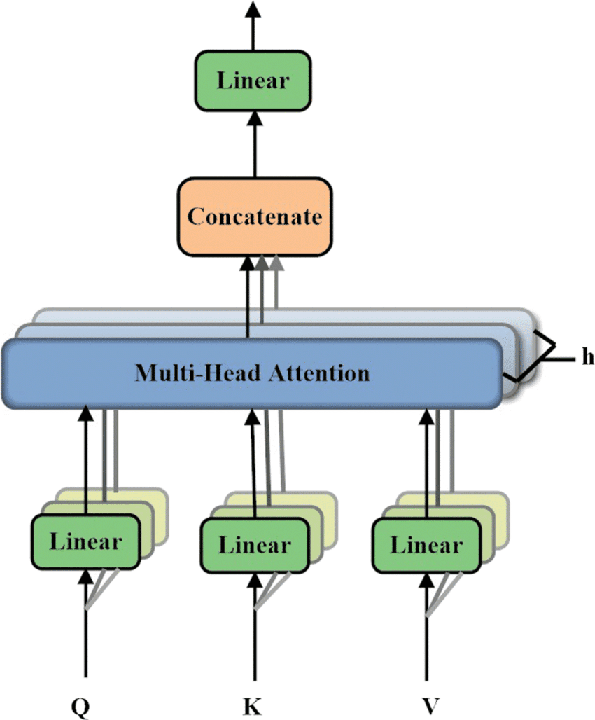
The transformer architecture
Let's study the original architecture, designed for sequence-to-sequence tasks.
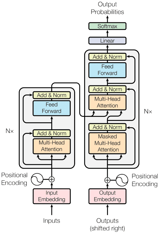 Positional encoding: Used to give the model a sense of the order of the input tokens, since the self-attention mechanism is inherently order-agnostic (unliKe RNNS). Self-attention treats the input sequence as a set and has no notion of token position unless explicitly provided.
In the original Transformer, positional encoding is added to the input embeddings:

 Each row represents a positional encoding - notice how none of the rows are identical!
Note: modern systems use learned positional embedding instead of sine-cosine-based ones. In this approach, the positional encodings become trainable parameters, similar to the word embeddings.
Add & Norm: Residual connections and layer normalization, crucial for stabilizing training and improving information flow.
MLP: Self-attention by itself is actually a linear operation, despite how it might seem at first. The non-linearity in the Transformer architecture comes from other components, like the activation functions (e.g., ReLU) in the feed-forward neural networks (MLPs), not from the self-attention mechanism itself.
Autoregression The encoder is used just once to encode the entire input. Then, the decoder is going to generate the output sequence one token at a time, using self attention with:
- The encoder output as Key and Value
- The queries come from the sentence generated so far
- actually, we still use learned weight matrices to generate the Queries (Q), Keys (K), and Values (V), but the inputs for these matrixes come from different sources.
Training and Masked self attention The first self-attention mechanism in the decoder is masked to ensure that the model generates output in a causal or auto-regressive manner.
During training, the model has access to the entire target sequence. If the self-attention mechanism were not masked, the model could "cheat" by looking ahead at future tokens that it is supposed to predict, leading to information leakage.
During training in a Transformer model, the loss is calculated using the predicted tokens generated by the decoder compared to the ground truth target sequence. At each time step, the decoder processes the input token (the previous ground truth token, forced teaching) and generates a probability distribution over the vocabulary for the next token.
The total loss for the entire sequence is computed by summing the loss across all time steps.
