Glossary of layers used in Deep Learning

Introduction
Deep learning architectures are built using layers that perform specific and often simple tasks. It is essential for any machine learning practitioner to have a solid understanding of the different types, functionalities, and purposes of these layers.
I have compiled a concise summary of the most common layers used in deep learning models, and I often refer back to it to refresh my memory and review details. This summary uses PyTorch implementations as references.
The following table provides an overview of the layers and elements that this post will cover:
| Layer | Description |
|---|---|
nn.Linear | This layer implements a fully connected (dense) layer, where each neuron is connected to every neuron in the previous and next layers. |
nn.Conv2d | Implements the standard 2D convolution operation, where a filter (also known as a kernel) slides over the input data and computes the dot product between the filter weights and the corresponding input value. Used for downsampling the input data, extracting features, and learning spatial hierarchies. |
nn.ConvTranspose2d | Also known as transposed convolution or deconvolution, performs an upsampling operation by applying a learnable upsampling filter to the input data. |
nn.MaxPool2d / nn.AvgPool2d | Pooling for downsampling. |
nn.ReLU / nn.Sigmoid / nn.Tanh | Activation functions necessary for introducing non-linearity to the network and enabling better gradient flow. |
nn.BatchNorm2d / nn.LayerNorm | Normalization techniques used to improve the training stability and speed up convergence by normalizing the input to each layer; can also reduce overfitting. |
nn.Embedding | Used for learning embeddings in natural language processing (NLP) tasks. It maps discrete categorical variables (such as words or tokens) to continuous vector representations. |
nn.LSTM / nn.GRU | These layers implement Long Short-Term Memory (LSTM) and Gated Recurrent Unit (GRU) cells, which are popular choices for modeling sequential data. |
nn.Softmax / nn.LogSoftmax / nn.Sigmoid / nn.Tanh / Identity | Functions used at the last layer for different types of tasks: nn.Softmax and nn.LogSoftmax for multi-class classification, nn.Sigmoid for binary classification, nn.Tanh for regression tasks where output is expected to be within a specific range, and Identity for raw output in regression tasks. |
nn.CrossEntropyLoss / nn.MSELoss / nn.BCELoss | Provides various loss functions. |
Fully Connected Layers
A fully connected (dense) layer, implemented in PyTorch as nn.Linear, is one of the most fundamental building blocks in neural networks. Each neuron in a fully connected layer is connected to every neuron in the preceding and following layers. This means that every output value is influenced by every input value, allowing for complex interactions.
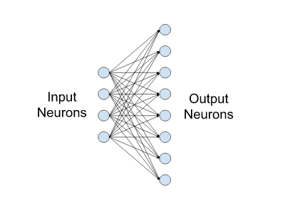
Fully connected layers are excellent at combining features extracted from previous layers. For example, after a series of convolutional layers, a fully connected layer can combine these features to make a final prediction.
💡 Insight: The main purpose of fully connected layers is to learn complex representations of the input data by combining features in a non-linear fashion.
A word of caution: despite their versatility, fully connected layers are computationally expensive, especially when dealing with large input sizes. Each neuron in a fully connected layer has a weight associated with every neuron in the previous layer, leading to a large number of parameters. To mitigate these issues, fully connected layers are often used sparingly and strategically within modern architectures. For example, they are typically placed at the end of convolutional networks, where the input size has been significantly reduced by earlier layers.
Convolutional Layers
2D Convolutions
This is the most common convolution, implemented in PyTorch as nn.Conv2d, it performs a convolution operation on input data, typically images. This layer uses a set of learnable kernels that slide over the input data to extract features such as edges, textures, and shapes. Each kernels is convolved with the input, producing a feature map that highlights the presence of specific features at different spatial locations.
 The following animation from the paper A guide to convolution arithmetic for deep learning exemplifies the application of a 3x3 filter to a single-channel feature map:
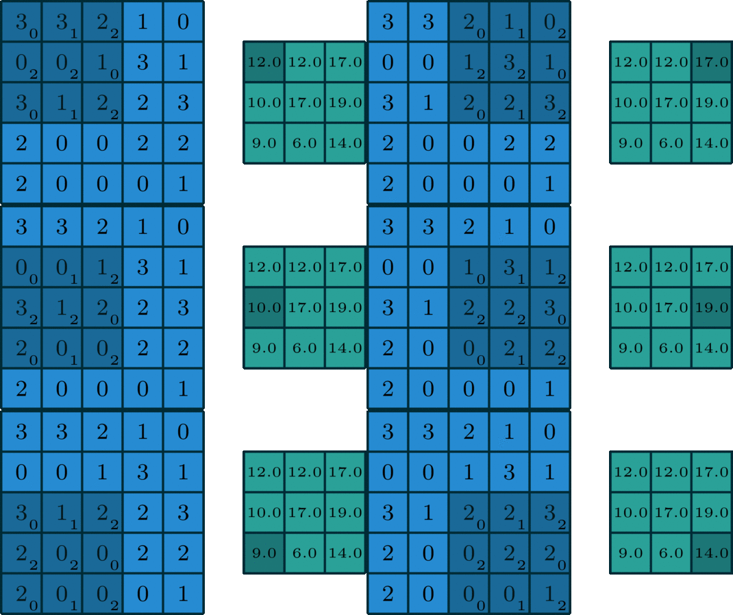
The words "kernel" and "filter" are often ambiguously used as synonyms, but the distinction becomes really important when the convolutional layer receives a multi-channel output and outputs a multi-channel output as well:
- Kernel: A kernel is a small matrix (e.g., 3x3, 5x5) that slides over a single channel of the input data to perform the convolution operation. Each kernel captures local patterns in the input.
- Filter: A filter is composed of multiple kernels, one for each channel in the input. For example, if the input has three channels (as in an RGB image), a filter will have three corresponding kernels. Each kernel slides over its respective channel in the input, and the results of all the individual kernels are summed to produce the output of the filter. This summed output is a single channel feature map.
💡 Example: ResNet-50 applies a 2D convolution in its first layer. The input of the layer is a 224x224x3 RGB image, and a 7x7 convolution reduces it into a 112x112x64 feature map. In order to output 64 feature maps, the convolution employs 64 kernels, each one having 3 learnable filters of size 7x7.
There are plenty of reasons why convolutional layers are so popular:
- 2D convolutions excel in capturing spatial hierarchies of features within images. They can detect low-level features like edges and textures in early layers, gradually learning higher-level features such as shapes and objects in deeper layers. This hierarchical feature extraction is crucial for tasks like image classification, object detection, and segmentation.
- Unlike fully connected layers, where each neuron is connected to every input neuron, 2D convolutions use a shared set of parameters (kernels). This parameter sharing significantly reduces the number of learnable parameters, making the network more efficient and easier to train. This is a ground-breaking improvement!
- They are customizable by many parameters such as stride and padding, which allow practitioners to choose how to manipulate the input data appropriately.
- Convolutional architectures have proven effective across a wide range of computer vision tasks, showing great generalization.
On the other hand, convolutions have its limitations:
- Each neuron in a convolutional layer has a fixed receptive field determined by the kernel size. This fixed size may limit the model's ability to capture global context or larger patterns that span across the entire input, especially in tasks where global information is crucial. This is why transformer architectures sometimes are able to surpass convolutional architectures.
- The hierarchical nature and abstraction of features learned by deep CNNs can sometimes make it challenging to interpret how and why the model makes specific predictions
💡 Example: Object detection in cluttered scenes is a situation where an architecture based on convolutional layers may struggle, because multiple objects may overlap or occlude each other. This requires integrating information across large spatial extents or understanding complex relationships between objects. Here, a transfomer-based architecture may be more suitable
Please check out the post Intuitively Understanding Convolutions for Deep Learning for a thoroughly detailed yet intuitive explanation of convolutions.
💡 Insight: Convolutional layers can be stacked together to learn hierarchical features from images, making them a powerful tool for extracting rich features. They are way more efficient than fully connected layers because they only have to learn the parameters of small kernels
Transposed Convolutions
Transposed convolutions, implemented in Pytorch as nn.ConvTranspose2d, are used to upsample (increase the spatial resolution of) a feature map. They achieve this by adding neighboring values in the input layer, weighted by a convolution matrix. This process effectively reverses the downsampling performed by regular convolutions, making it useful for tasks like image generation and semantic segmentation.
This great example from "Understand Transposed Convolutions" provides an intuition for a 2x2 single channel input, which is upsampled via a 3x3 transposed convolution to a 3x3 single channel output.
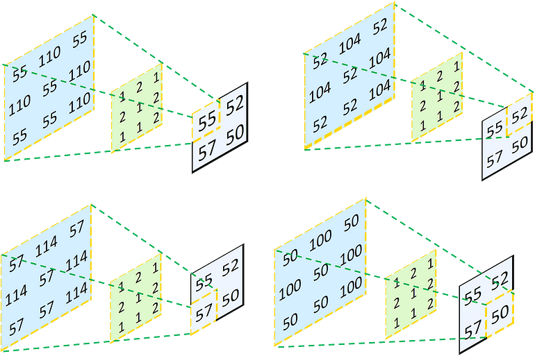
First, each element in the input layer is multiplied by each value in the kernel (green). Then, the resulting layers (in blue) are added element-wise to produce a 3x3 output. Naturally, the exact same numbers are not restored. The kernel parameters are learned to get better results.
Transposed convolutions are often called deconvolutions, and are implemented in Pytorch as nn.ConvTranspose2d
1x1 convolutions
1x1 convolutions are a specialized form of 2D convolution where the kernel size is 1. They may seem a pointless at first, with such a small receptive field one cannot really learn any spatial patterns from the input. Nevertheless, they do offer several significant advantages:
- Dimensionality Reduction: They allow for mapping an input feature map with depth N to an output feature map with depth
M<N, effectively reducing the number of channels. - Channel-Wise Information Exchange: They facilitate the exchange of information between channels, enhancing feature interactions.
- Efficiency: Due to the small kernel size, 1x1 convolutions are computationally efficient, requiring fewer parameters to learn.
💡 Example: Popular architectures like ResNet and Inception extensively utilize 1x1 convolutions for their efficiency and ability to transform feature dimensions.
 Image from "A Comprehensive Introduction to Different Types of Convolutions in Deep Learning"
Atrous Convolutions
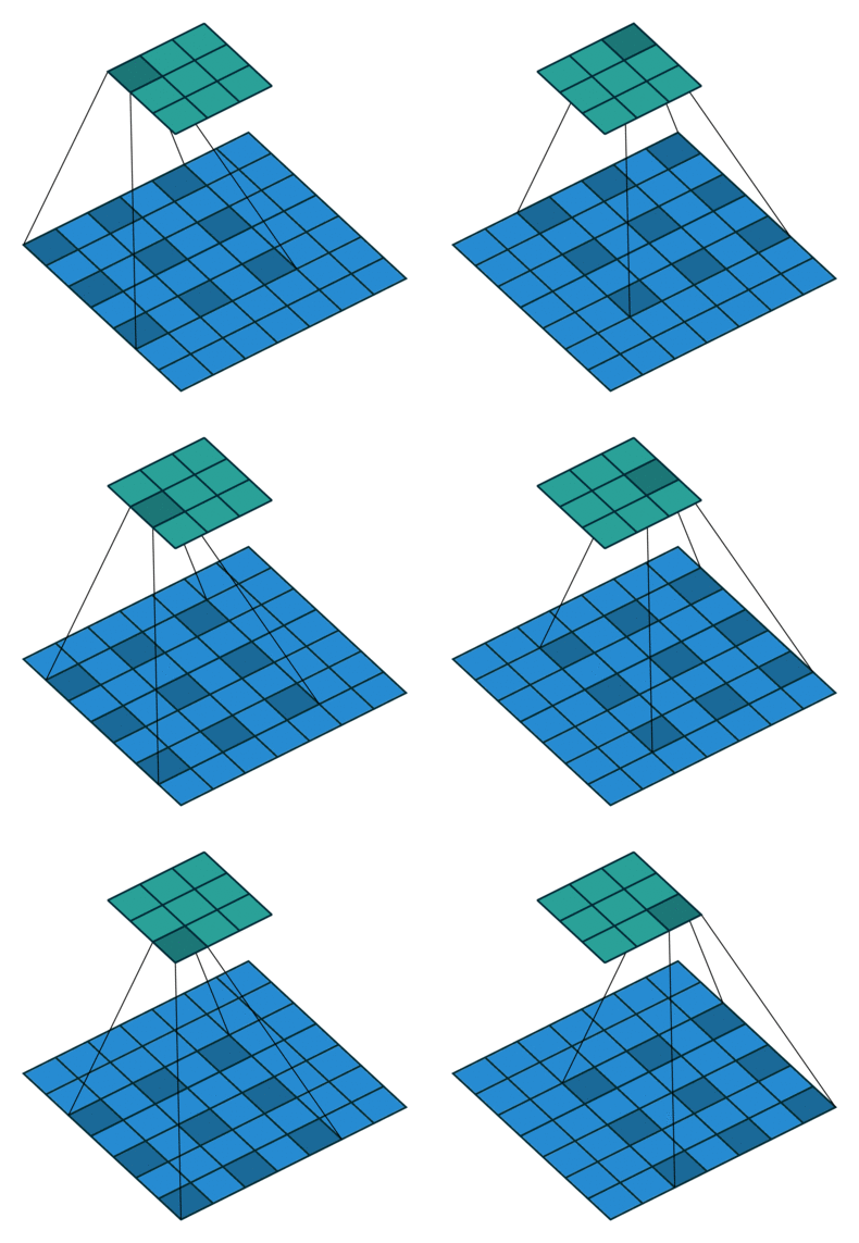
Also known as dilated convolutions, these convolutions expand the effective receptive field by inserting holes between kernel elements, controlled by a dilation rate parameter. This technique enables the network to capture spatially distant features more effectively without downsampling through pooling operations.
3D Convolutions
2D convolutions do perform convolution on 3D inputs, but a key distinction here is that each filter depth is the same as the input layer depth (depth being the number of channels).
A 3D convolution is a generalization of a 2D convolution, where the filter depth is smaller than the input layer depth, and the filter slides in all 3 dimentions (height, width and channels of the image)
 Image from "A Comprehensive Introduction to Different Types of Convolutions in Deep Learning"
Pooling Layers
Like convolutional layers, pooling operators use a fixed-shape window that slides over the input regions based on its stride, computing a single output for each location covered by the window (often referred to as the pooling window). However, unlike convolutional layers, which perform cross-correlation between inputs and kernels, pooling layers contain no parameters (no kernel). Instead, pooling operators are deterministic, typically computing either the maximum or average value of the elements within the pooling window. These operations are known as maximum pooling (max-pooling) and average pooling, respectively.
 Image from Deep Neural Networks on Chip - A Survey
When handling multi-channel input data, the pooling layer processes each input channel independently, unlike convolutional layers that sum the inputs across channels. As a result, the number of output channels in the pooling layer remains the same as the number of input channels.
A few implications of using pooling are:
- The combination of convolutional and pooling layers facilitates hierarchical feature learning and reduces the spatial dimensions of the data.
- The dimensionality reduction (downsampling) makes the network faster and more efficient.
- Pooling layers inherently lose information and fine-grained details. Max pooling, for example, discards potentially important information.
💡 Insight: In a convolutional network, the deeper we go, the larger the receptive field (relative to the input) to which each hidden node is sensitive. Pooling layers expedite this process by reducing spatial resolution, allowing the convolution kernels to cover a larger effective area.
Note: Global Average/Max Pooling is a type of layer often used to reduce the data from each channel to a single value. It's simply using a filter size = (W,H)
Activation Layers
Activation layers introduce non-linearity into the network, enabling it to learn complex patterns. Without activation functions, the network would essentially behave like a linear regression model, regardless of its depth. Here are some of the most commonly used activation functions in deep learning:
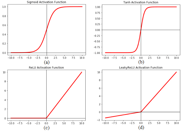
In Pytorch, convolutional layers do not apply activation function by default. One has to manually add activation layers (nn.ReLU / nn.Sigmoid / nn.Tanh) typically applied after each convolutional layer and fully connected layer. They are not applied after pooling layers.
| Use Case | Activation Function | When to Use | Why | Drawbacks |
|---|---|---|---|---|
| General Use | ReLU | Default choice for hidden layers in most neural networks | Efficient computation, mitigates vanishing gradient problem, works well in practice | Can lead to dead neurons (neurons may stop learning) |
| Binary Classification | Sigmoid | Output layer for binary classification tasks | Outputs values between 0 and 1, interpretable as probabilities | Can cause vanishing gradients, computationally expensive |
| Multi-class Classification | Softmax | Output layer for multi-class classification tasks | Outputs a probability distribution over classes, with probabilities summing to 1 | Not suitable for hidden layers |
| Zero-centered Data | Tanh | Hidden layers when zero-centered outputs are desired | Output ranges from -1 to 1, helping in centering the data | Can cause vanishing gradients, computationally expensive |
💡 Benefits of ReLU: You will notice that most models choose ReLU as their activation function. This is due to many benefits:
- Its gradient is either 0 or 1, which helps maintaining stronger gradients during backpropagation, allowing for faster and more effective training
- It outputs either 0 for negative values, creating sparsity in the activations, which can improve network performance and reduce computation
- Other activation functions involve exponential calculations, which are computationally expensive.
💡 Insight: Without activation functions, the entire neural network would collapse into a single linear function, making it unable to learn from data with non-linear patterns.
At this point, we can look at how these basic layers are chained into a very simple CNN for classification into 10 classes (e.g. MINST digit classification):
import torch
import torch.nn as nn
import torch.nn.functional as F

class SimpleCNN(nn.Module):
    def __init__(self, num_classes):
        super(SimpleCNN, self).__init__()
        self.conv1 = nn.Conv2d(in_channels=3, out_channels=16, kernel_size=3, padding=1)
        self.pool = nn.MaxPool2d(kernel_size=2, stride=2, padding=0)
        self.conv2 = nn.Conv2d(in_channels=16, out_channels=32, kernel_size=3, padding=1)
        self.fc1 = nn.Linear(in_features=32 * 8 * 8, out_features=128)
        self.fc2 = nn.Linear(in_features=128, out_features=num_classes)

    def forward(self, x):
        x = self.conv1(x)
        x = F.relu(x)
        x = self.pool(x)
        x = self.conv2(x)
        x = F.relu(x)
        x = self.pool(x)
        x = x.view(-1, 32 * 8 * 8)  # Flatten the tensor
        x = self.fc1(x)
        x = F.relu(x)
        x = self.fc2(x)
        return x

# Example usage
model = SimpleCNN(num_classes=10)
print(model)Normalization
Normalization generally refers to techniques that adjust the scale of input data to a standard range, often between 0 and 1 or with a mean of 0 and variance of 1. The goal is to improve the convergence of optimization algorithms and prevent features with larger numerical ranges from dominating those with smaller ranges.
Within a deep neural network such as the SimpleCNN shown above, activation layers such as ReLu produce activations on its neurons. As we train the network, the distribution of these activations changes constantly due to weight updates, a phenomenon known as internal covariate shift. This internal covariate shift can slow down the convergence of the network, make the training process less stable, and make the model more sensitive to the choice of hyperparameters such as the learning rate.
💡 Insight: Internal covariate shift can cause the computed gradients to be unstable, leading to vanishing or exploding gradients. Inconsistent activation distributions can slow down convergence as well, requiring more iterations to learn meaningful representations. Think of it as learning a "moving target", that's really hard. The main goal of normalization is to transform these activations so that they fall within a more standardized range. With fixed activations, we can increase the learning rate and speed up the convergence.
Normalization layers are designed to overcome the issue of internal covariate shift. Let's make this very explicit with a toy example. Say we consider the activations of two training samples A and B at a certain layer within a deep neural network.
-
Without Normalization:
- Training Sample A: Activations might be in the range of
[100, 200, 300]. - Training Sample B: Activations might be in the range of
[1, 2, 3].
- Training Sample A: Activations might be in the range of
-
With Normalization:
- Adjust activations to have a mean of zero and standard deviation of one.
- After normalization:
- Training Sample A: Activations might be transformed to
[0.5, 1, 1.5]. - Training Sample B: Activations might be transformed to
[-0.5, 0, 0.5].
- Training Sample A: Activations might be transformed to
This normalization ensures that the activations from different training samples are within a common range, making the training process more stable and efficient. The network can then learn more effectively, as the optimization process is dealing with a more predictable and controlled range of activation values.
Batch Normalization
During training, we usually take mini batches out of the training dataset, of small size (e.g. 8 or 16), feed them to the network, calculate the loss, calculate the gradient and update the weights. We perform one weight update for the entire mini batch.
Batch normalization is a technique introduced to address the issues caused by internal covariate shift. It normalizes the output of a previous activation layer by subtracting the batch mean and dividing by the batch standard deviation. This normalization is followed by scaling and shifting using learnable parameters.
The following snippet is a good summary of this:
def BatchNorm(x, gamma, beta, eps=1e-5):
  """
  BatchNorm performs batch normalization on input x.

  Args:
      x: Input data of shape (N, C, H, W).
      gamma: Scale factor of shape (1, C, 1, 1).
      beta: Shift factor of shape (1, C, 1, 1).
      eps: A small epsilon value for numerical stability (default: 1e-5).

  Returns:
      The normalized input of shape (N, C, H, W).
  """
  # Calculate mean and variance of the input across all except channel dimension
  mean = x.mean(dim=[0, 2, 3], keepdim=True)
  var = x.var(dim=[0, 2, 3], keepdim=True)

  # Normalize the input
  x_hat = (x - mean) / torch.sqrt(var + eps)

  # Scale and shift the normalized input
return x_hat * gamma + betaApplying batch normalization with minibatches of size 1 would result in no learning at all because subtracting the means would leave each hidden unit with a value of 0. The method proves effective and stable only with sufficiently large minibatches. This highlights the importance of batch size when using batch normalization; proper calibration or adjustment of batch size is crucial for optimal performance.
💡 Consideration: Typically, after training, we use the entire dataset to compute stable estimates of the variable statistics and then fix them at prediction time. Hence, batch normalization behaves differently during training than at test time. Recall that dropout also exhibits this characteristic.
Layer Normalization
Unlike batch normalization, which normalizes across the batch dimension, layer normalization normalizes across the features for each individual training example. This makes it particularly useful for recurrent neural networks (RNNs) and situations where batch sizes are small or vary.
Layer normalization operates by normalizing the summed inputs to the neurons within a given layer. The following snippet can provide a good intuition:
import tensorflow as tf

def LayerNorm(x, gamma, beta, eps):
  """
  Layer normalization function.

  Args:
    x: Input tensor.
    gamma: Scale factor learnable parameter.
    beta: Shift learnable parameter.
    eps: A small constant to prevent division by zero.

  Returns:
    Normalized tensor.
  """
  # Calculate mean and variance across channels, height, and width
  mean = tf.reduce_mean(x, axis=[1, 2, 3], keepdims=True)
  variance = tf.reduce_mean(tf.square(x - mean), axis=[1, 2, 3], keepdims=True)

  # Normalize
  norm_x = (x - mean) / tf.sqrt(variance + eps)

  # Scale and shift
return gamma * norm_x + betaGiven an input tensor x with shape (batch_size, height, width, channels), the mean and variance are reduced across the height, width, and channels dimensions, resulting in the mean and variance having the shape (batch_size, 1, 1, 1).
In other words, for every sample, we get a single scalar mean and variance (no distinction between channels), and we substract and divide elementwise. Then we have two learnable parameters gamma and betta used to scale and shift, just like for batch normalization.
Comparison
The following table summarises the key points:
| Aspect | Batch Normalization | Layer Normalization |
|---|---|---|
| Normalization Method | Across the batch | Across the features for each sample |
| Requires Large Batch Size | Yes | No |
| Suitability for CNNs | Very good | Less effective |
| Suitability for RNNs/Transformers | Less effective | Very good |
| Inference Behavior | Uses moving averages of mean and variance | Consistent behavior as in training |
| I also find the illustration for the post Build Better Deep Learning Models with Batch and Layer Normalization to be of great help when it comes to understanding the differences: |
 Batch normalization
 Layer normalization
Embedding layers
Embedding layers are a foundational component in natural language processing (NLP), and are commonly used in transformer architectures.
They are designed to convert discrete categorical variables into continuous vectors, effectively mapping items (such as words) into a high-dimensional space. This mapping captures semantic relationships between items, facilitating tasks like word prediction, classification, and clustering.
Concretely, an embedding layer is a lookup table where each entry corresponds to a vector representation of a unique item from the input space. For example, in the context of text, each word in the vocabulary is assigned a unique vector. These vectors are learned during training and capture the semantic meaning of words based on their usage in the training data.
Recurrent layers
Recurrent layers are fundamental for processing sequential data, such as time series, text, and audio. They enable neural networks to maintain information about previous elements in a sequence, capturing temporal dependencies and contextual information. The two most commonly used recurrent layers are Long Short-Term Memory (LSTM) and Gated Recurrent Unit (GRU).
The last layer
The final layer in a neural network is crucial for producing the desired output format, whether it's for classification, regression, or another task. Different activation functions serve different purposes, and selecting the right one is key to achieving good performance.
Final Layers Summary
| Activation Function | Use Case | Characteristics | Typical Usage Example |
|---|---|---|---|
nn.Softmax | Multi-class classification | Converts logits to probabilities that sum to 1 | Image classification with multiple classes |
nn.Sigmoid | Binary or multi-label classification | Maps output to (0, 1) range | Binary classification, multi-label classification |
nn.Tanh | Regression or bounded outputs | Maps output to (-1, 1) range | Regression tasks requiring bounded outputs |
nn.Identity | No activation required | Passes input directly as output | Conditional activations, certain output layer setups |