View Synthesis of Indoor Environments from Low Quality Imagery

Introduction
In my previous post, I introduced Neural Radiance Fields (NeRFs)—a technique for synthesizing realistic images from novel viewpoints, given a set of training images with camera pose annotations.
This time, I’m taking the theory into practice by training several NeRF variants on images of my own 60 m² apartment. You’ll see detailed reconstructions of rooms and objects, demonstrating the impressive capabilities of these methods.
To push the boundaries of what NeRFs can handle, I introduced challenging constraints on the training data. For instance, one dataset consists solely of images captured very close to the floor (z=5 cm), while another uses low-resolution images restricted to a fixed height plane (z=175 cm). These setups simulate real-world limitations often encountered in fields like robotics, where data collection can be constrained by environment or equipment.
NeRFs are typically designed and tested on small-scale objects, so scaling them to larger and more intricate scenes is a significant challenge. Despite the constraints I imposed in my experiments, the results were surprisingly robust, demonstrating the potential of NeRFs to perform well under practical limitations.
In addition to these experiments, I’ll explore advanced NeRF variants that incorporate natural language processing (NLP) prompts for tasks requiring semantic understanding of the environment. As a bonus, I’ll compare NeRFs to a classical alternative: Gaussian Splatting, offering a more efficient alternative.
Data Collection
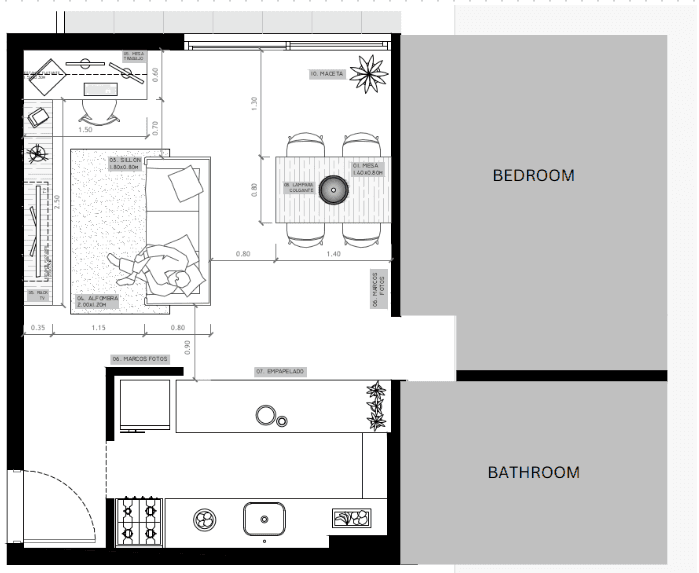
Let's quickly go over the two datasets that I collected for these experiments. Below you can see a plane of my apartment, where I collected video using an iPhone 14.

- For dataset 1, I walked around holding the phone in my forehead, capturing video for about 3 minutes from different viewpoints. I was always facing forward, meaning that the camera poses should roughly lie at
z=1.75meters and at a fixed angle around thexandyaxis. - For dataset 2, I attached the phone to a wheeled toy at a height 5 cm from the floor. I moved the camera around the home, capturing footage from a very low viewpoint. Again, there was no rotation along the
xandyaxis.
After extracting the individual frames from each video, the resulting datasets are:
| Dataset | Height | Number of Images | Camera settings | Original Resolution |
|---|---|---|---|---|
| Dataset 1 | ~175 cm | 6962 | 0.5X zoom | 1080x1920 |
| Dataset 2 | ~5cm | 8823 | 0.5X zoom | 1080x1920 |
Across the experiments you will notice that I reduced the resolution significantly to test the limits of NeRF when data quality is not good.
Camera Pose Estimation
This is the trickiest step in the process, and perhaps the most critical one. For most NERF methods to work, not only do we need a training dataset of images, but also their 3D camera positions. Intrinsic camera parameters are also required.
For the purposes of this post, let's assume that no prior knowledge of camera poses is available. In an upcoming post, I will be discussing how to integrate prior pose knowledge, e.g. from a SLAM system or iPhone's Polycam.
Colmap is the standard tool used to estimate the poses of a set of overlapping images, and I found that most NERF implementations assume people have run Colmap on their data before training.
Colmap can be very finicky, often failing without providing any hint of what is wrong. It is crucial to clean up your dataset as much as possible and provide the proper settings to the different colmap commands. I wrote a detailed appendix with a step-by-step description on how to use colmap.
If everything went fine, you should now have a sparse model specifying the camera poses of each image in your dataset, as well as the intrinsics of your camera. We are ready to train NeRFs!
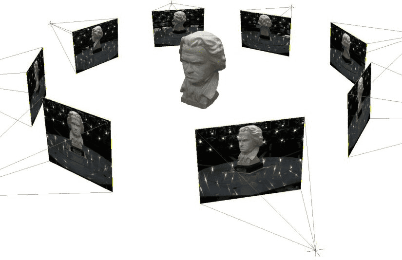
 3D poses of my training dataset images estimated by Colmap
Training NeRFs
After exploring a handful of implementations, I came across NeRFStudio , which conveniently implements a wide variety of cutting-edge NeRF methods:
- Intuitive API for training, rendering videos.
- Well documented and maintained.
- It works perfectly with Viser in order to navigate the 3D reconstruction.
- Supports tracking with W&B.
A couple of practical comments about training NeRFs - A detailed guide is included in appendix II:
- Training is very fast, even for larger scenes. In my experiments, it takes up to 30 minutes to fully train a NeRF using 4 NVIDIA GeForce RTX 2080 GPUs.
- Training quickly converges to a sensible reconstruction. If you didn't get a roughly accurate reconstruction after 2-3 minutes, then something is off.
- Training can be memory intensive, if you run out of memory consider reducing the batch size or reducing image resolution.
As of metrics, I will mostly use pixel-wise rgb loss and PSNR (Peak Signal-to-Noise Ratio). Human supervision can catch many details that aggregated stats do not represent.
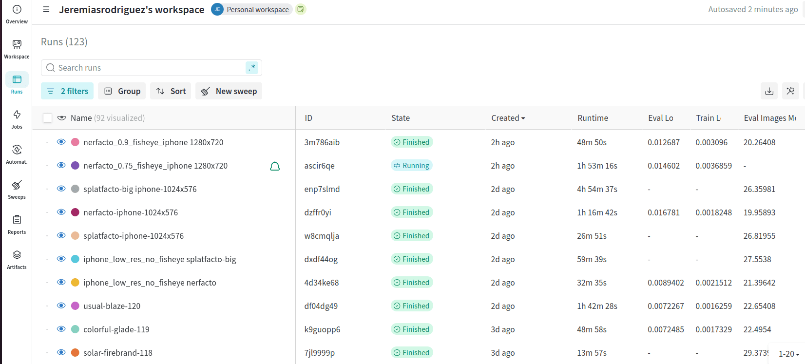
Tip: Use W&B to track and tag your experiments. NERFs can be trained very fast, and it is easy to lose track of each execution.

Nerfacto
The star method implemented by NeRFStudio is nerfacto, which takes the best ideas of recent innovations in the field and fuses them into a single implementation. In my experience, nerfacto provides the most realistic reconstructions for real-world data, and it is widely used as the default choice by practitioners in the field.
In the introduction you can watch a video from a trained Nerfacto on Dataset 1 at full resolution. The following video showcases Nerfacto trained on Dataset 2 at 0.5 resolution.
The following reconstruction is a NeRF on a sparser version of Dataset 1>
Notice that all images in these videos are synthetic, and the trajectory features many viewpoints not included in the training dataset. The ability to generate novel views from arbitrary camera positions is what makes NeRFs so powerful.
The NeRFs from Dataset 1 struggle to generate views for z much higher or much lower than 1.75m ; whereas the NeRF from Dataset 2 struggles to generate views higher vantage points. This is due to the training data being restricted to 1.75 m and 0.05 m respectively.
As stated before, the training loss quickly converges, with only marginal improvements after the first thousand of iterations:

W&B provides a convenient way to inspect the rgb and depth reconstruction evolution of specific validation images at different iterations.

At times I am mesmerized by the details that the NeRF is able to encode in its weights:
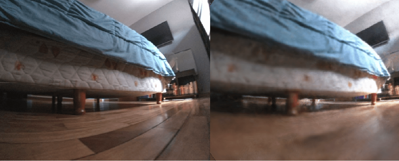
 A NeRF trained on very low res images (430x760) is able to learn the mattress pattern, as well as details of individual books on a shelf.
 A NeRF trained on low resolution images (540x960) is able to learn the wooden floor pattern in detail. Notice the accurate reconstruction of the TV screen and the map in the wall.
 *A NeRF trained on 540x960 images is able to perfectly learn the mirror reflection. The mirror reflection is adjusted as the viewpoint changes.
A small fraction of the dataset is set aside for validation. Different status, such as PSNR, can be calculated on the reconstructed-original image pairs. PSNR was around 23 for Dataset 1 and 26 for Dataset 2 on their respective validation datasets.

Splatfacto
A traditional yet much more efficient alternative to NeRF is Gaussian Splatting. It can be trained even faster than NeRFs, uses up considerably less memory, and occasionally produces better results.
For the demo video below I used Splatfacto, which is conveniently implemented in NeRFStudio. Given the reduced memory usage, I was able to train at full resolution and obtain an amazing reconstruction:
The following table summarizes a few key metrics, although comparing different columns is not really correct, given the differences in resolution and different holdout sets from Dataset 1 and Dataset 2.
| Metric | NeRF Dataset 1 (0.5x res) | NeRF Dataset 2 (0.4x res) | Gaussian Splatting Dataset 1 (0.8x res) |
|---|---|---|---|
| PSNR (dB) | 23 | 26 | 27 |
| SSIM | 0.85 | 0.88 | 0.90 |
| Training Time | 27 mins | 25 mins | 23 mins |
| Memory Usage | High | High | High |
Advanced NeRF variants
I spent quite a while playing with other NeRF variants, such as LERF (Language Embedded Radiance Fields). LERF introduced the CLIP concept to NeRFs, allowing the user to make text queries and producing an activation heatmap in response.
For instance, the relevancy map for "sofa" is:
 The relevancy map for "mirror":

Given the heavy memory requirements, I was only able to train a Lite version of LERF, which was capable of accurately handling queries for individual objects like "tv", "window", "shoes". However, the model struggled to understand more complex concepts like "a comfortable place to sit down".
Conclusion
In this blog post, I explored the application of NeRF and Gaussian Splatting models trained on severely restricted, low-resolution real-world images.
On the positive side, these techniques successfully captured the structure of the apartment, and in many cases, they were able to reconstruct fine details with impressive accuracy. Once the dataset is properly cleaned, these models are relatively quick and straightforward to train.
However, there are challenges. View synthesis models, particularly NeRF, can struggle to generate realistic views from unseen viewpoints. In the demo videos, NeRF exhibits hallucinations, creating bright, unrealistic shapes when the novel viewpoints deviate too far from the training data. Additionally, preparing an effective training dataset is no small feat, as outlined in Annex I.
Towards the end of the post, I briefly introduced LERF, a 2023 model that combines NeRF with natural language processing (NLP). The lightweight model I trained offers a glimpse into the exciting possibilities when a powerful representation like NeRF is merged with language models.
This emerging field is full of potential, and I am eager to see how it evolves in the coming years—there are undoubtedly many breakthroughs on the horizon!
Appendix I : How to run Colmap on custom data
First and foremost, a good clean dataset is the single most important factor to obtain a good reconstruction. Tips that I have learned in the last months are:
- Try to remove featureless images, such as closeups of walls, from your dataset.
- Try to expose the scene from as many viewpoints as possible.
- If possible, remove blurry images.
- Try to prevent too many dynamic objects, if possible have none.
- For the current SOTA methods, keep your dataset size bounded, don't go over 10K, images, ideally much less.
- For the current SOTA methods, don't try to reconstruct environments larger than
~100 m^2 - Consistent good lighting
- If you have too many duplicates or very high frame-rate, consider downsampling.
- Reconstruction quality degrades with low image resolution. Use the highest resolution possible.
- Make sure all images were obtained with the same camera, using the same settings ; and if possible research the camera model used.
Step 1: Feature Extraction
Ensure you first install the last version of colmap:
sudo apt install colmap
The first step is feature extraction, and involves detecting and describing keypoints (distinctive features) in each input image. These keypoints serve as the foundation for matching and estimating the relative positions of cameras and 3D points in the scene
Assuming that input images are stored in imgs folder, feature extraction can be run as follows:
colmap feature_extractor --database_path database.db --image_path imgs/ --ImageReader.single_camera 1 --SiftExtraction.use_gpu 1 --ImageReader.camera_model
The parameters provided are:
- --database_path: A location where a new database will be created, and the results of feature extraction (and subsequent steps) will be stored. Ensure that you remove an older database that may live in this same path.
- --image_path: A folder storing your training images
- --ImageReader.single_camera: We are forcing the model to assume all the images come from the same camera. This is not suitable if you change camera settings on the fly or if you are using images from different cameras.
- --SiftExtraction.use_gpu 1: Speed up using GPU. Later steps are actually going to take forever unless you use a GPU.
If you happen to know that your camera uses a specific camera model, and if you even happen to know the intrinsic parameters of your camera, then you should definitely input them to the feature extractor, e.g by adding these parameters to the command:
--ImageReader.camera_model OPENCV_FISHEYE --ImageReader.camera_params "281.08,282.98,319.51,236.08,0.01,-0.23,-0.27,0.19"
For the iPhone images with zoom 0.5X I used a RADIAL model, which is able to model the distortion caused by the zoom.
--ImageReader.camera_model RADIAL
The execution time of this step is very short, less than 2 minutes. After it finishes, colmap should have populated several tables on database.db. I strongly encourage you to sanity-check the database by inspecting it:
$ sqlite3 database.db
SQLite version 3.31.1 2020-01-27 19:55:54
Enter ".help" for usage hints.
sqlite> select count(*) from images;
8823
sqlite> select * from images limit 5;
1|1000.jpg|1
2|10002.jpg|1
3|10000.jpg|1
4|10001.jpg|1
5|10003.jpg|1
sqlite> select * from descriptors limit 5;
1|576|128|
2|462|128|
3|504|128|
4|449|128|
5|470|128|
)&There should be as many images in the images tables as there were in your folder, and both the .descriptors and .keyframes tables should have been populated. There should also be one entry in .cameras table.
Step 2: Feature Matching
In this computationally expensive step, colmap is going to try to match the features extracted in the previous step across multiple images. There are several strategies that can be used to reduce computation time, but I have opted for exhaustive matching which consistently ensures best results. Exhaustive matching scales very poorly to large image datasets, it can take hours for datasets with up to 10000 images, and I strongly encourage you to seek alternatives (such as sequential matching) if your dataset is larger.
Exhaustive matching can be run as follows:
colmap exhaustive_matcher --database_path database.db --SiftMatching.use_gpu 1
After it finishes, the table .matches should have been populated in your database.db
Step 3: Sparse Model Generation
The third and last step is to geometrically verify the matches and iteratively estimate the camera poses:
colmap mapper --database_path database.db --image_path imgs/ --output_path sparse --Mapper.ba_global_function_tolerance=1e-5
The parameter --Mapper.ba_global_function_tolerance=1e-5 governs one of the termination conditions, and I suggest trying 1e-6 to 1e-4 values depending on the quality of your data and the execution time you are willing to endure. This step can take several hours if you impose a very low tolerance and/or if your dataset is too large.
The results of this step will be, finally, estimations of your camera poses, stored in the subfolders of the sparse folder. Often, colmap will produce several alternative estimations, and store them in subfolders named sparse/0, sparse/1, sparse/2, etc.
The best one is supposed to be /0, however I have often found that /0 has been able to reconstruct the pose for very few points, and I end up using an alternative such as /1.
Let's discuss how to inspect and debug one of these reconstructions, e.g. /0. Inside one such folder, you should find three files:
- cameras.bin: Here are listed all the cameras (we actually constrained the problem to just one camera, so just one entry). For each camera, you'll find the estimated intrinsic paramaters.
- images.bin: Here are the estimated poses of each image that colmap managed to map. Notice that a few of the original images, sometimes the vast majority of them, may not have entries here meaning that colmap failed to estimate their pose.
- points3D.bin: Points in the scene that colmap has seen across several images, and their triangulated pose.
Actually, in order to read the contents of these files, I encourage you to convert the bin files into txt files as follows:
colmap model_converter --input_path /sparse/0 --output_path /sparse/0 --output_type TXT
If your ultimate goal is to train NERFs, the most important part is to check the fourth line of images.txt, which may say something like this:
# Number of images: 8725, mean observations per image: 497.11243553008597
This indicates the number of images whose pose has been estimated. Aim at this number being a significant proportion of your original dataset, ideally >90%. If your dataset has too many featureless frames, I've seen this number degrade quickly, even to values as low as 3% and the output model only matching featureless frames amongst themselves.
If sparse/0 has too low a proportion of poses estimated, checkout sparse/1, since previous iterations of the mapper may have arrived at decent reconstructions.
Colmap has a GUI that you can use to load and visualize a sparse model. I will be showcasing NeRFStudio visualizer later on though, which is much better to visualize your estimated camera poses.
Step 4: Refine Poses
Optionally, you may try to refine your camera pose and intrinsics estimates even further. In my experience this can run for too long and produces unnoticeable results, but I suppose it must be helpful in some situations because systems like NeRFStudio do this by default:
colmap bundle_adjuster --input_path sparse/0 --output_path sparse/0 --BundleAdjustment.refine_principal_point 1
Appendix II: NeRFStudio
In order to train NeRF using NeRFStudio, you must first create a conda environment and setup NeRFStudio. The official instructions work seamlessly, I suggest you install from source so that you can edit the scripts as needed.
The next step is to convert colmap estimated poses into NeRFStudio input format:
ns-process-data images --data ./colmap/imgs --output-dir .
This will generate a transforms.json file listing the camera poses as homogeneous transforms.
In order to train nerfacto, you can run:
ns-train nerfacto --data DATA_FOLDER --output-dir OUTPUT_FOLDER --vis=viewer+wandb
Where:
- Data folder is the folder where transforms.json and images are located
- Output folder is where the trained model will be stored
There are literally hundreds of parameters that you can provide to ns-train, you can see the list (and very lazy descriptions) by running ns-train nerfacto -h.
If you are running out of memory, you can try reducing memory consumption by sacrificing training speed by using settings like:
--steps-per-eval-batch 200 --pipeline.datamanager.train-num-rays-per-batch 1024 --pipeline.datamanager.eval-num-rays-per-batch 1024
If you are still out of memory, or if you want to reduce the resolution of your images before training, use:
--pipeline.datamanager.camera-res-scale-factor 0.5
Finally, I have found that disabling pose optimization can often lead to best reconstructions:
--pipeline.model.camera-optimizer.mode off
During training, you will be provided with an address to run Viser on a browser. This visualization is likely going to be very rough due to latency and the model being updated live.
You can navigate the reconstruction as though you were playing a FPS game. Use WASDQE and the arrows to navigate in all 3 dimensions. Create viewpoints and click on "generate command" to save a trajectory which can be then rendered in full resolution after training:
ns-render camera-path --load-config CONFIG_PATH --camera-path-filename CAMERA_PATH --output-path renders/nerfstudio.mp4
You can use other models by picking one out of the list enumerated in ns-train -h. I encourage you to try splatfacto-big which is much very efficient and not as resource heavy as NeRF.
As a final piece of advise, track your experiments with W&B since you can easily train hundreds of reconstructions while trying out models and parameters.