Introduction to Semantic Segmentation using MMSegmentation

Overview

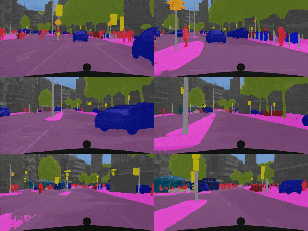
In this post, I will introduce a specific computer vision task called semantic segmentation and a toolbox for training and evaluating semantic segmentation models called MMSegmentation.

Using the benchmark dataset Cityscapes, I will provide a step-by-step guide on how to train and evaluate your own semantic segmentation model. Additionally, I will demonstrate how to use a trained model to make predictions with my own original dataset of street-view images from Rosario, Argentina.

Semantic Segmentation 101

Semantic Segmentation is a computer vision task that consists of categorizing each pixel of an input image into one of a finite set of classes:

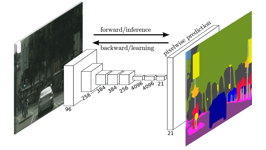
This sample belongs to Cityscapes, one of the most popular benchmark datasets for semantic segmentation. This dataset contains about 25k street-view pictures of European cities, along with pixel-level classification for 29 classes such as road, bike, sidewalk and sky.

Semantic segmentation is extremely useful to help computer systems understand and reason about their environment in a global way. It provides granular information on the semantics of an image. Popular applications include:

Semantic Scene Understanding: This is valuable for intelligent robots and autonomous vehicles, which need to understand visual scenes in order to make sensible decisions (e.g., navigating in complex environments).

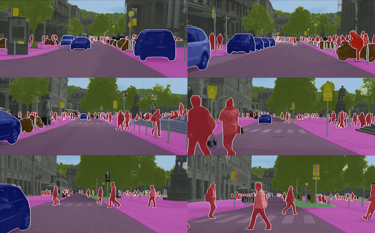Source: Robot Learning Lab, University of Freiburg

Healthcare: In medical diagnostics, semantic segmentation is revolutionizing patient care by providing precise measurements and analyses of medical imagery..

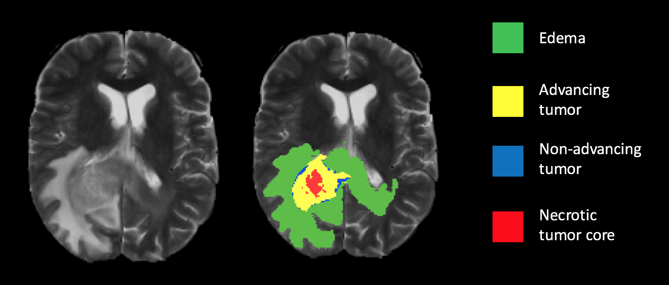Early detection of brain tumours - Source

Aerial image processing: Applicable to a wide variety of tasks such as surveillance, agriculture monitoring, urbane planning, forest management, etc.

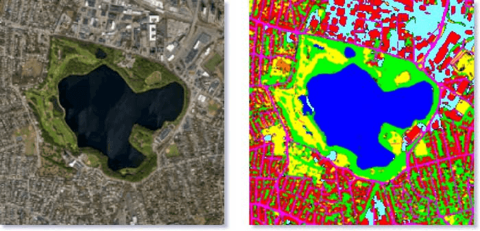Segmentation of satellite imagery - Source

Solving Semantic Segmentation

Typically, this problem is tackled using supervised learning, where a machine learning model is trained on a dataset of images annotated at the pixel level. This task is inherently more challenging than image classification, which aims to predict a single label for an entire image.

State-of-the-art semantic segmentation models require a substantial amount of annotated data, which is more expensive to acquire compared to the labels needed for image classification or even object detection.

I compare popular segmentation architectures, including UNet, PSPNet and DeepLab, in this separate post.

Pyramid Scene Parsing Network (PSPNet) - Source: Original paper

In this post, I will introduce MMSegmentation as a convenient and reliable way to train these models, using Cityscapes as the running example.

MMsegmentation

Mmsegmentation is an extraordinarily well documented and high-quality toolbox that greatly simplifies training and evaluating semantic segmentation models. It provides:

• High-quality libraries, so you don't need to reimplement basic procedures.
• The most popular architectures already implemented and ready to use.
• Flexibility to be used with any dataset, custom architecture, metric or loss function.
• PyTorch-based implementation.
• Well documented and open source

Mmsegmentation is part of OpenMMLAB, a broader toolkit that provides support for virtually all mainstream computer vision tasks.

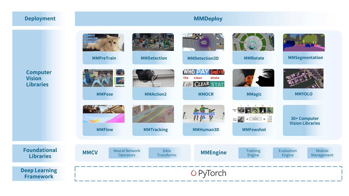
Setting up MMSegmentation

Let’s jump straight into the task of training a semantic segmentation model using one of the Cityscapes datasets. As with any ML project, the first step is to use conda to create an isolated environment where we can safely have our own package installations:

conda create --name semseg_first_experiment python=3.8 -y
conda activate semseg_first_experiment

The next step is to install MMsegmentation. Check the official installation guide for the most up-to-date steps, which as of today and assuming you have local GPUs available are:

conda install pytorch torchvision -c pytorch
pip install -U openmim
mim install mmengine
mim install "mmcv==2.1.0"
git clone -b main https://github.com/open-mmlab/mmsegmentation.git
cd mmsegmentation
pip install -v -e .

At this point, the MMSegmentation repo is cloned and ready to go. The size of the codebase may seem a little daunting at first, but you only need to be aware of a few crucial files to start training basic models. Here I summarise them:

• mmsegmentation/data: This is where all datasets should live, including the input images and the target segmentation masks. By default, it's empty, so you must take care to download and move the data you want to use.
• mmsegmentation/tools/dataset_converters: Standalone scripts that are used to convert the data into the appropriate format for training.

💡 Tip: Input images are expected to be RGB images in jpg or png format, whereas target segmentation masks should be single-channel images, with classes encoded as ascending integer values.

• mmsegmentation/tools/dist_train.sh : A convenient script to train a model on multiple GPUs.
• mmsegmentation/tools/dist_test.sh : A convenient script to test a model on multiple GPUs.
• mmsegmentation/mmseg/models: This is where the actual PyTorch models are defined.
• mmsegmentation/mmseg/datasets: Dataset class definitions for all supported datasets, defining the target classes, evaluation metrics, path suffixes, etc.
• mmesgmentation/configs: All config files should go here, governing the settings and parameters for any given machine experiment.
• mmsegmentation/work_dirs: By default, training stats, model checkpoints, and visualizations are stored here.

Training Cityscapes

First, the training and validation Cityscapes data must be downloaded. To do so, the owners of the dataset require users to make an account at https://www.cityscapes-dataset.com/. Then, the data can be downloaded as follows:

wget --keep-session-cookies --save-cookies=cookies.txt --post-data 'username=YOUR_EMAIL&password=YOUR_PASSWORD&submit=Login' https://www.cityscapes-dataset.com/login/; history -d $((HISTCMD-1))
wget --load-cookies cookies.txt --content-disposition https://www.cityscapes-dataset.com/file-handling/?packageID=1
wget --load-cookies cookies.txt --content-disposition https://www.cityscapes-dataset.com/file-handling/?packageID=3

Replace YOUR_EMAIL and YOUR_PASSWORD with your newly created credentials. The downloaded files must be unzipped and moved to mmsegmentation/mmseg/datasets/cityscapes.

The next step is to preprocess the raw data, transforming the segmentation masks to the appropriate format that MMsegmentation expects. There is a handy script already provided in the repo:

python tools/convert_datasets/cityscapes.py data/cityscapes --nproc 8

MMsegmentation has already defined the Dataset, evaluation metrics and different flavors of config files for Cityscapes.

• mmsegmentation/mmseg/datasets/cityscapes.py: Defines file suffixes and visualization palette.
• mmsegmentation/configs/_base_/datasets/cityscapes.py : Base config file of the dataset, specifying:
  • Train and validation pipelines. Here is where different preprocessing steps such as resizing, cropping and data augmentation are specified.
  • The paths from which the data will be loaded.
  • The batch_size, which will affect how much memory your GPUs will require.
• mmsegmentation/configs/pspnet/pspnet_r101-d8_4xb2-80k_cityscapes-512x1024.py: One of the many provided config files, which I picked for this tutorial. This one specifies:
  • Model : PSPNet
  • Depth: 101 layers
  • Number of iterations: 80k
  • Network input size: 512 x 1024
  • Default optimizer SGD, default learning rate policy
  • Many more settings

Training can now be started as follows:

./tools/dist_train.sh configs/pspnet/pspnet_r101-d8_4xb2-80k_cityscapes-512x1024.py 4

Here, 4 is the number of GPUs in my case (set this to the number of GPUs you have available for training, which may be just 1).

Analizing Training and Validation Results

Training may take a few days depending on your hardware. MMsegmentation will periodically print the iteration number and the training loss. As your model learns from the training examples, you will see the training loss value go down:

2024/05/13 22:58:17 - mmengine - INFO - Iter(train) [   50/40000]  lr: 9.9891e-03  eta: 16:31:08  time: 0.8793  data_time: 0.0053  memory: 10445  loss: 2.1633  decode.loss_ce: 1.4961  decode.acc_seg: 41.6312  aux.loss_ce: 0.6672  aux.acc_seg: 47.5072
2024/05/13 22:59:01 - mmengine - INFO - Iter(train) [  100/40000]  lr: 9.9779e-03  eta: 13:05:37  time: 0.8761  data_time: 0.0055  memory: 6112  loss: 2.1990  decode.loss_ce: 1.5059  decode.acc_seg: 41.6787  aux.loss_ce: 0.6930  aux.acc_seg: 46.6241
2024/05/13 22:59:45 - mmengine - INFO - Iter(train) [  150/40000]  lr: 9.9668e-03  eta: 11:56:17  time: 0.8740  data_time: 0.0062  memory: 6112  loss: 1.9273  decode.loss_ce: 1.3541  decode.acc_seg: 82.7501  aux.loss_ce: 0.5732  aux.acc_seg: 70.7805

💡 Tip: When training on your own GPUs, use tmux to run the training script in a detached terminal so that it keeps running in the background and it doesn't get accidentally interrupted. This is vital if you're remotely accessing your GPU machine.

Validation stats will be calculated and printed every 4000 iterations, and a checkpoint of the model weights will be saved in mmsegmentation/work_dirs. The validation loss will give an insight into the generalization capabilities of the model over unseen data.

For this particular example, after 80k iterations, the training loss has gone down significantly, which indicates that the model has been able to learn from the training data:

07/07 14:04:20 - mmengine - INFO - Iter(train) [80000/80000]  lr: 1.0000e-04  eta: 0:00:00  time: 1.2293  data_time: 0.0081  memory: 9595  loss: 0.1310  decode.loss_ce: 0.0888  decode.acc_seg: 96
.7349  aux.loss_ce: 0.0421  aux.acc_seg: 96.3267

💡 Tip: If your training loss does not go down, then the model is not learning at all! As a safety check, I always first train my models using a handful of samples from the training set both as the training and validation set. Your model should be able to easily memorize these samples, otherwise there is something wrong.

Validation stats look like this after 80k iterations:

07/07 14:05:41 - mmengine - INFO - 
+---------------+-------+-------+
|     Class     |  IoU  |  Acc  |
+---------------+-------+-------+
|      road     |  98.3 | 99.03 |
|    sidewalk   | 85.86 | 92.77 |
|    building   | 93.04 | 96.81 |
|      wall     | 51.61 | 56.01 |
|     fence     | 62.39 |  71.6 |
|      pole     | 67.72 | 81.96 |
| traffic light | 74.38 | 86.64 |
|  traffic sign | 81.14 | 88.77 |
|   vegetation  | 92.82 | 96.77 |
|    terrain    | 63.53 | 71.44 |
|      sky      | 94.98 | 98.18 |
|     person    | 83.66 | 93.46 |
|     rider     | 65.28 | 78.07 |
|      car      | 95.49 | 98.23 |
|     truck     | 80.36 |  84.3 |
|      bus      | 83.65 | 93.12 |
|     train     | 58.12 | 59.03 |
|   motorcycle  | 69.27 | 77.07 |
|    bicycle    | 79.32 | 89.94 |
+---------------+-------+-------+
07/07 14:05:41 - mmengine - INFO - Iter(val) [125/125]    aAcc: 96.3100  mIoU: 77.9400  mAcc: 84.9100  data_time: 0.0072  time: 0.6070

Intersection over Union (IoU) is a standard metric for semantic segmentation, which describes how much the predicted segmented regions of each class overlap with its ground truth. We can see, for example, that this model is quite good at predicting road whereas it struggles a little more to predict train or wall. This is not surprising, as the latter two are rare and underrepresented in the training data. Often, the solution is to add more labeled data to the training set to reduce the imbalance.

To monitor and visualize training stats, I like to use TensorBoard, which will make handy plots such as:

The smoothed loss value as a function of the number of iterations

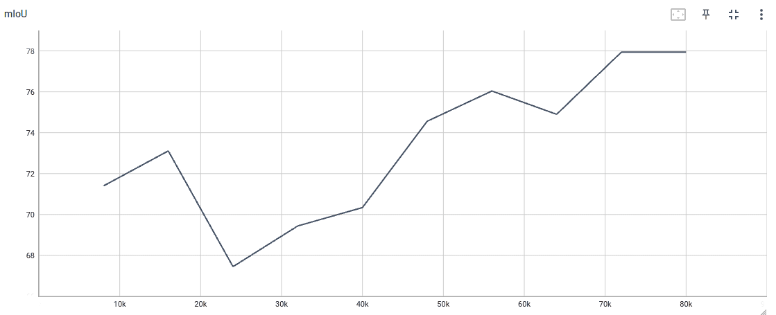The validation performance (avg. IoU) as a function of the number of iterations

💡 Tip: From this plot, we can see that the model may still keep improving if we let it train for more than 80k iterations. Training must be allowed to go on until improvement stagnates.

I also like to save the model predictions as images during validation to see what the network is predicting and how that changes over time. To do this, you should modify your scheduler. For this example, set the following default hook in mmsegmentation/configs/_base_/schedules/schedule_80k.py.

    visualization=dict(type='SegVisualizationHook', draw=True, interval=1))

This will save images in your mmsegmentation/work_dirs . For example, let's see what our model was predicting early in training:

4000 iterations. left: ground truth - right: model prediction

40k iterations. left: ground truth - right: model prediction

Notice that the segmentation after 40k iterations is clearly better than the prediction after only 4k iterations.

:memo: Note: Most models, PSPNet included, load backbone pretrained weights by default. This means that they will try to leverage pre-trained weights that have been learnt from larger datasets such as ImageNet. If you wish to disable the use of pretrained models, you may do so by setting the key pretrained=None in your model in your config file.

Evaluating Your Trained Model on Custom Datasets

After finishing training, you will find all the checkpoints of your model saved during validation as .pth files in the corresponding subfolder at mmsegmentation/working_dirs. These .pth files store the state dictionary of a model, which includes all the weights and biases. The config file of a model along with its state dictionary can be used to make inferences on new data.

To demonstrate this, I have compiled a small test set of images from my hometown Rosario (Argentina). I was curious to see whether the trained model would generalize well to images from South America, given that the training data comes exclusively from European cities.

In order to evaluate the model on a custom test set, there are two options.

1. If you have labels for your test data and you want to get statistics on the model performance, you may use ./tools/dist_test.sh as follows:
   • Move the test set to the appropriate data subfolder, such as `/mmsegmentation/data/cityscapes/custom_test_set
   • Set the path of the test dataset in the dataset config file mmsegmentation/_base_/datasets/cityscapes.py, under the test_dataloader key
   • Run ./tools/dist_test.sh {config file} {checkpoint} {num-gpus} --show-dir {output-visualization-folder}
2. If you have a set of images on which you want to perform segmentation using a trained model, and you simply want to make inferences, MMSegInferencer provides a convenient interface:

from mmseg.apis import MMSegInferencer
 
config_path = "work_dirs/pspnet_r101-d8_4xb2-80k_cityscapes-512x1024/pspnet_r101-d8_4xb2-80k_cityscapes-512x1024.py"
checkpoint_path = "work_dirs/pspnet_r101-d8_4xb2-80k_cityscapes-512x1024/iter_80000.pth"
image_folder = "data/cityscapes/argentina_test_set"
 
# Load model into memory
inferencer = MMSegInferencer(model=config_path, weights=checkpoint_path)
 
# Make inferences
inferencer(image_folder, out_dir='outputs', img_out_dir='vis', pred_out_dir='pred')

I opted for option (2) to generate predictions on the test set of images that I compiled from my hometown. I was pleasantly surprised to find that the trained segmentor makes sensible predictions in this unfamiliar setting, given that I devoted very little time to tuning the model. Let's go over a handful of predictions:

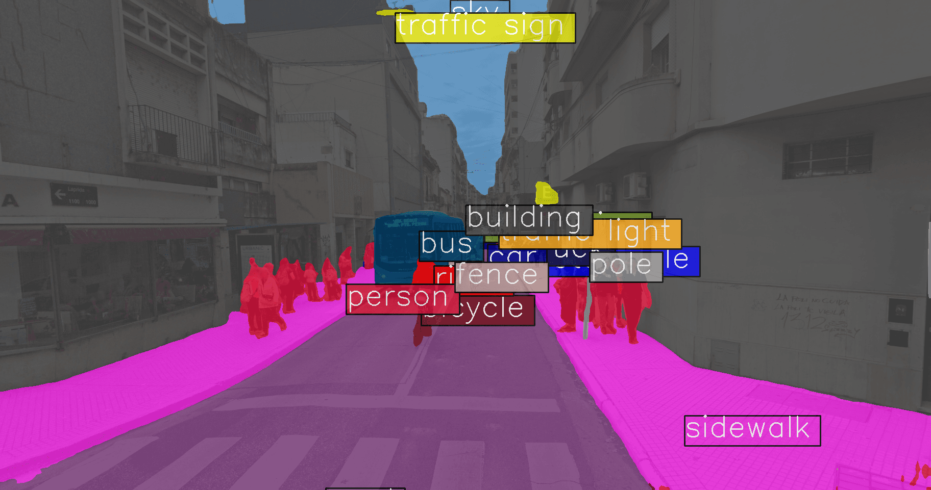The model managed to understand this complex scene quite accurately.

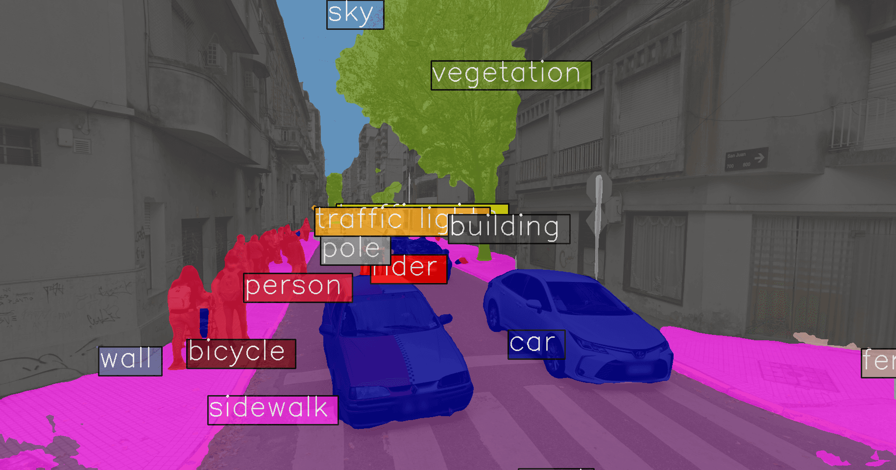The model managed to understand this scene quite accurately.

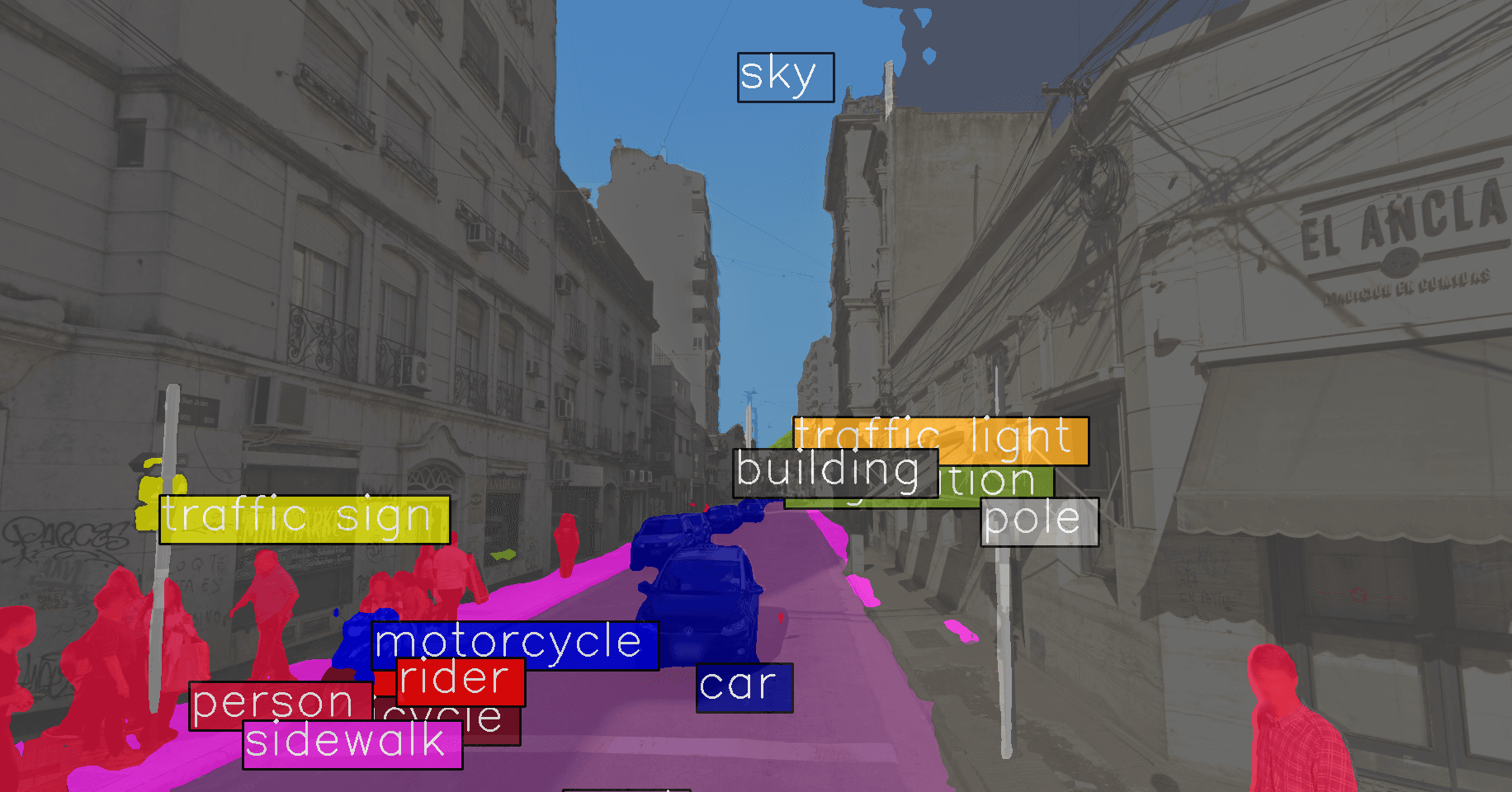The model managed to understand this scene quite accurately.

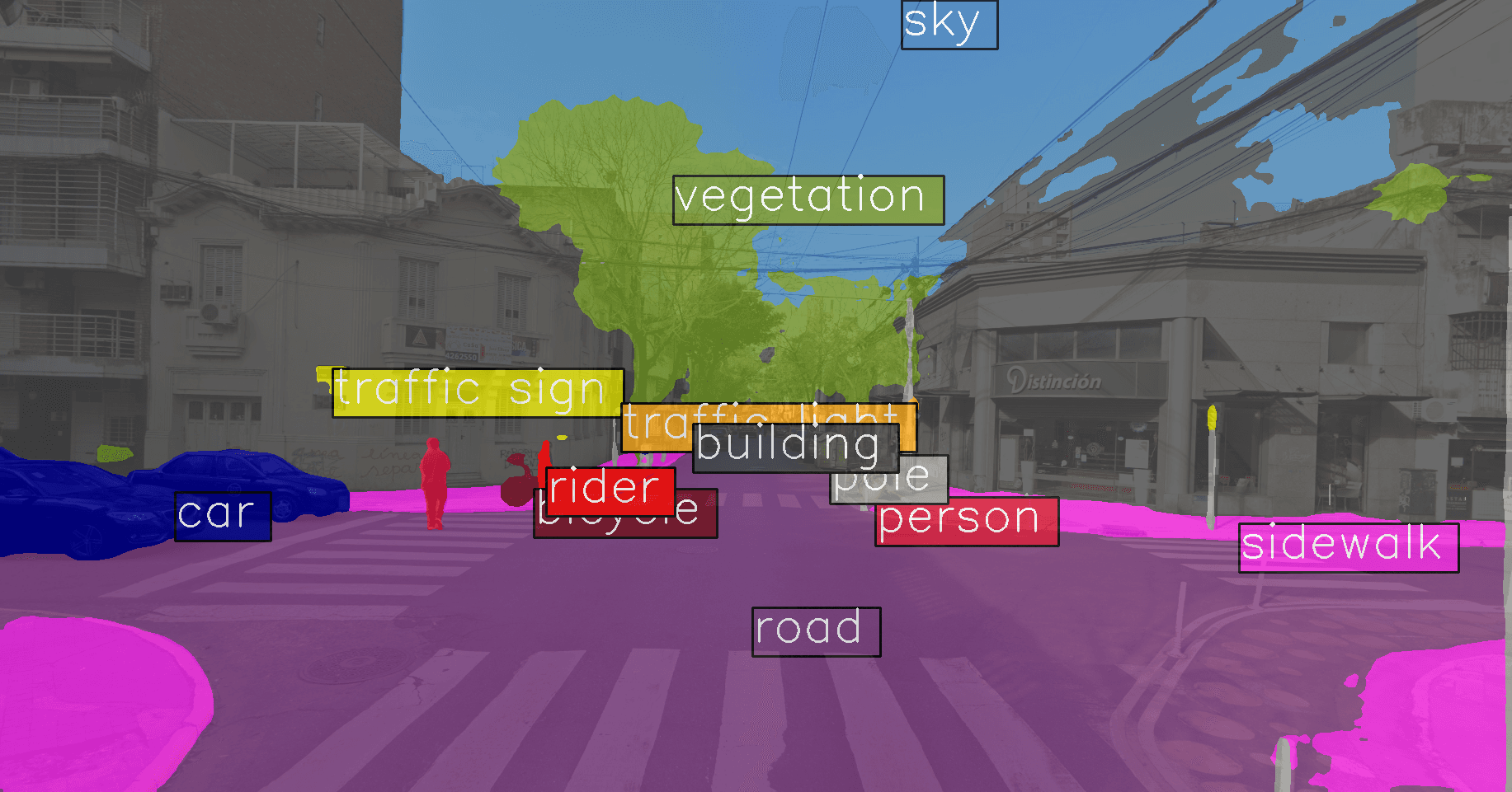Notice how the model inaccurately predicts part of the bike lane as "sidewalk" and part of the sky as "buildings". The untidy aerial hanging wires in the sky do confuse the model, something that is not likely seen in many European cities.

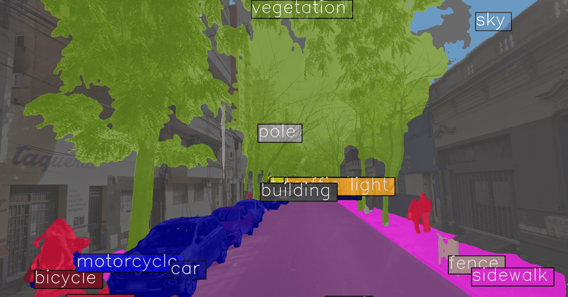Accurate prediction. I'm particularly impressed by the precise detection of vegetation.

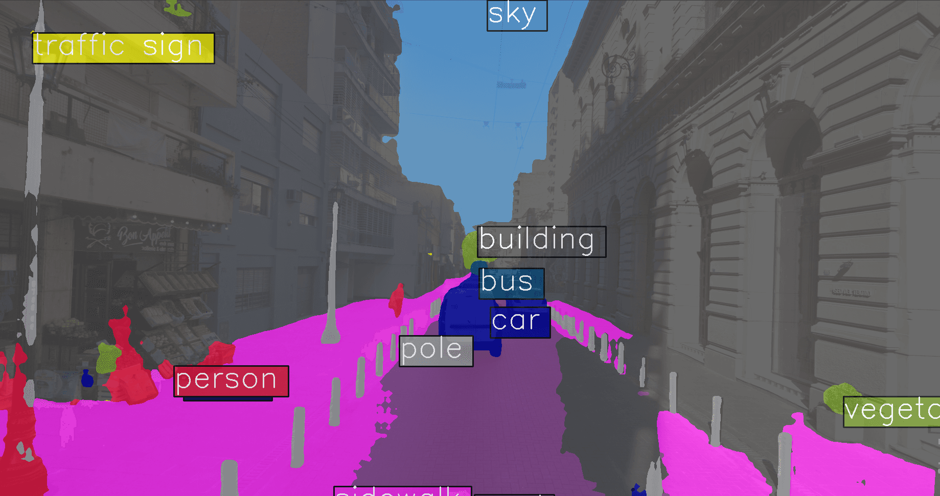This instance is quite a failure. The road and sidewalk in front of "Teatro El Circulo" are partially classified as building, and the left side of the road is considered to be sidewalk. The materials, textures and colors of this scene are relatively uniform, which may play a role in misleading the model. Notice the ghost person predictions on the left, another funny artifact.

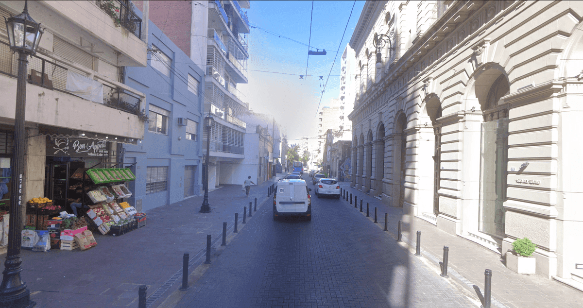The input image of the last prediction.

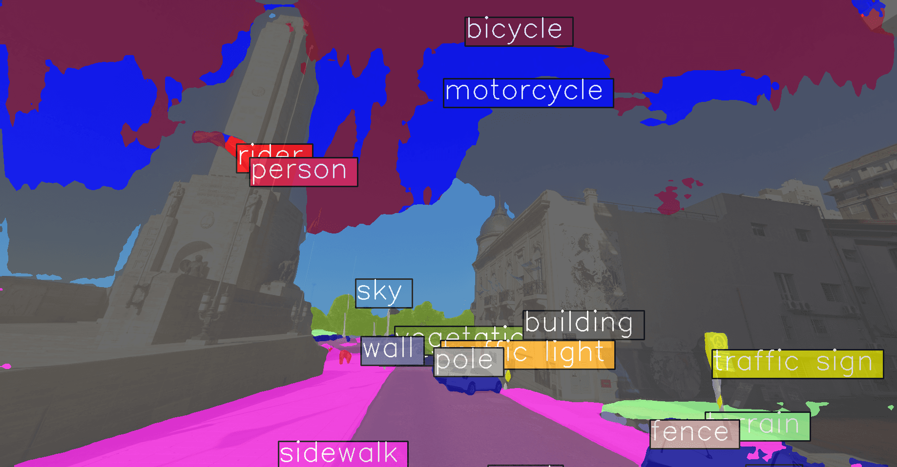This prediction exemplifies the often puzzling back-box nature of neural networks. Overall, this scene is well segmented, except for the sky, which for some reason has been predicted as being motorcycle and bicycle classes. It is usually not possible to get an explanation from the trained model of what prompted it to make such far-fetched choices for the sky area.

Conclusion

In this post, I introduced the task of semantic segmentation and highlighted its diverse applications across various domains. I presented MMSegmentation, an advanced toolbox designed for training segmentation models.

I outlined the steps to set up the MMSegmentation repository and demonstrated a complete training schedule using the Cityscapes dataset as an example. The training process spanned two days and resulted in achieving a mean Intersection over Union (mIoU) of 77.94 using a PSPNet with a reduced schedule of only 80k iterations. Visualizations and metrics showcased the model's capability to approximate the segmentation task.

Furthermore, I explained how to perform inference with a trained model and introduced an original test set from my hometown. This test set posed a challenge due to its data distribution differing somewhat from the training set. Despite this, the segmentations obtained were robust and sensible.

This post serves as an introduction to the concepts and framework utilized in my ongoing project, semantic segmentation for underwater scenery. Feel free to explore it further!

Pictures I took during my diving trip in Rangiroa, French Polynesia

Segmentation mask of the underwater scenery dataset I developed